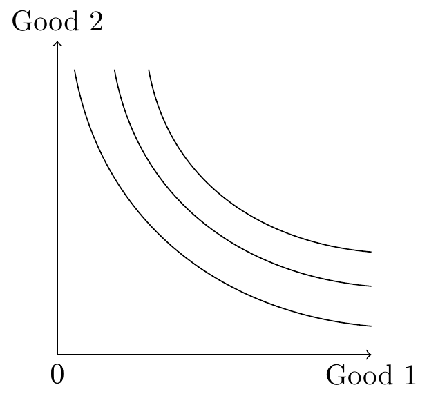
Indifference Curve

\begin{tikzpicture}[scale=.7]
% Axis
\draw [->] (0,0) node [below] {0} -- (0,0) -- (5.5,0) node [below] {Good 1};
\draw [->] (0,0) node [below] {0} -- (0,0) -- (0,5.5) node [above] {Good 2};
% Indifference curve
\draw (0.3,5) to [out=280,in=175] (5.5,0.5);
\draw (1,5) to [out=280,in=175] (5.5,1.2);
\draw (1.6,5) to [out=280,in=175] (5.5,1.8);
\end{tikzpicture}
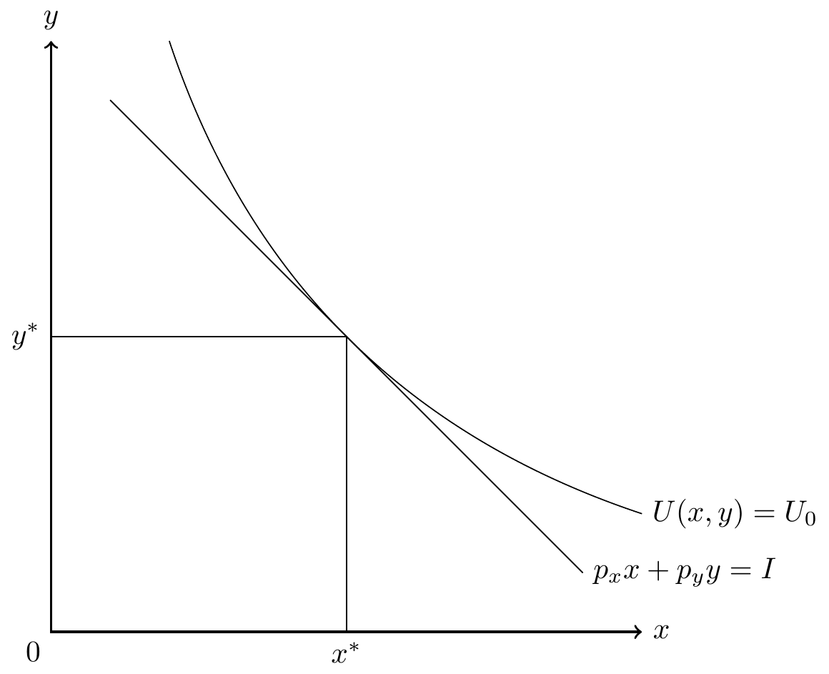
Utility Maximization

\begin{tikzpicture}[scale=.7]
\draw[thick,<->] (0,10) node[above]{$y$}--(0,0)--(10,0) node[right]{$x$};
\node [below left] at (0,0) {$0$};
\node [below] at (5,0) {$x^{*}$};
\node [left] at (0,5) {$y^{*}$};
\draw(1,9)--(9,1) node[right]{$p_xx+p_yy=I$};
\draw(0,5)--(5,5)--(5,0);
\draw(2,10) ..controls (3.33,6) and (6,3.33) .. (10,2) node[right]{$U(x,y)=U_0$};
\end{tikzpicture}
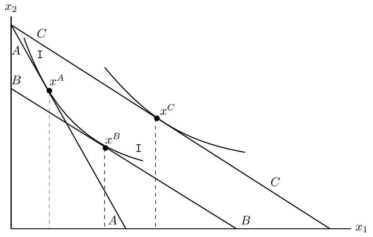
Hicks Decomposition

\begin{tikzpicture}[scale=1.2]
\draw [thick] (0,0) -- (8,0);
\draw [thick] (0,0) -- (0,5);
\node [right] at (8,0) {$x_1$};
\node [above] at (0,5) {$x_2$};
\draw [thick] (2.2,3.8) to [out=310,in=170] (5.5,1.8);
\draw [thick] (0.3,4.5) to [out=290,in=165] (3.1,1.6);
\node [right] at (6,1.1) {$C$};
\node [right] at (0.5,4.1) {$\texttt{I}$};
\draw [thick] (0,4.8) -- (7.5,0);
\draw [thick] (0,4.8) -- (2.7,0);
\draw[dashed](0.9,3.2)--(0.9,0);
\draw[dashed](3.4,2.6)--(3.4,0);
\draw [thick] (0,3.3) -- (5.3,0);
\draw[dashed](2.2,1.9)--(2.2,0);
\node [above] at (2.4,1.9) {$x^B$};
\draw[fill] (2.22,1.9) circle [radius =0.06];
\node [above] at (3,1.7) {$\texttt{I}$};
\node [right] at (0.8,3.5) {$x^A$};
\draw[fill] (0.9,3.25) circle [radius =0.06];
\node [right] at (3.4,2.8) {$x^C$};
\draw[fill] (3.43,2.6) circle [radius =0.06];
\node [right] at (0.5,4.6) {$C$};
\node [right] at (-0.1,4.2) {$A$};
\node [left] at (2.6,0.2) {$A$};
\node [right] at (5.3,0.2) {$B$};
\node [right] at (-0.1,3.5) {$B$};
\end{tikzpicture}
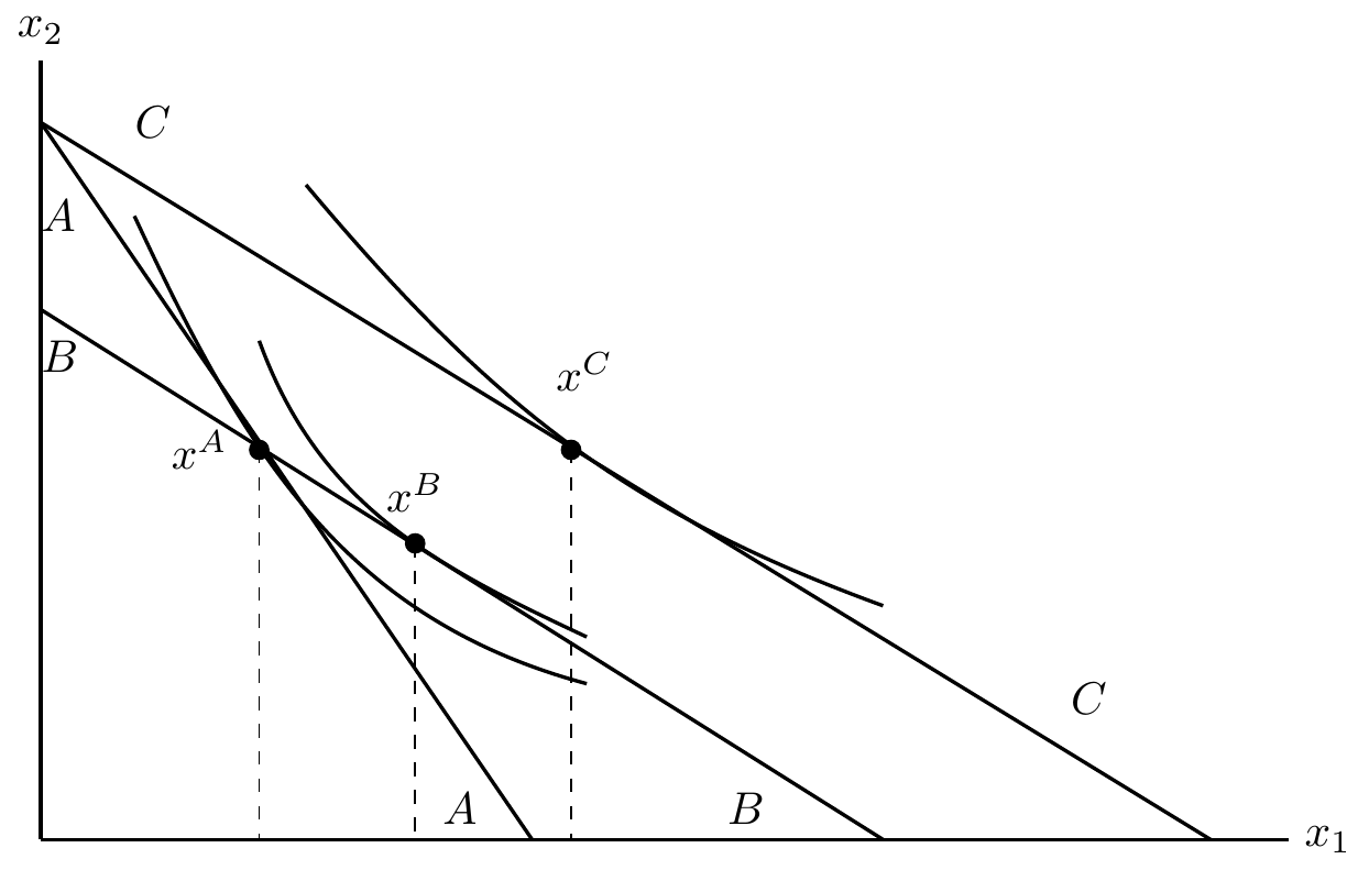
Slustsky Decomposition

\begin{tikzpicture}[scale=1.2]
\draw [thick] (0,0) -- (8,0);
\draw [thick] (0,0) -- (0,5);
\node [right] at (8,0) {$x_1$};
\node [above] at (0,5) {$x_2$};
\draw [thick] (1.7,4.2) to [out=310,in=160] (5.4,1.5);
\draw [thick] (0.6,4) to [out=295,in=165] (3.5,1);
\draw [thick] (1.4,3.2) to [out=290,in=155] (3.5,1.3);
\node [right] at (6.5,0.9) {$C$};
\draw [thick] (0,4.6) -- (7.5,0);
\draw [thick] (0,4.6) -- (3.15,0);
\draw[dashed](1.4,2.5)--(1.4,0);
\draw[dashed](3.4,2.5)--(3.4,0);
\draw [thick] (0,3.4) -- (5.4,0);
\draw[dashed](2.4,1.9)--(2.4,0);
\node [above] at (2.4,2) {$x^B$};
\draw[fill] (2.4,1.9) circle [radius =0.06];
\node [left] at (1.3,2.5) {$x^A$};
\draw[fill] (1.4,2.5) circle [radius =0.06];
\node [right] at (3.2,3) {$x^C$};
\draw[fill] (3.4,2.5) circle [radius =0.06];
\node [right] at (0.5,4.6) {$C$};
\node [right] at (-0.1,4) {$A$};
\node [left] at (2.9,0.2) {$A$};
\node [right] at (4.3,0.2) {$B$};
\node [right] at (-0.1,3.1) {$B$};
\end{tikzpicture}
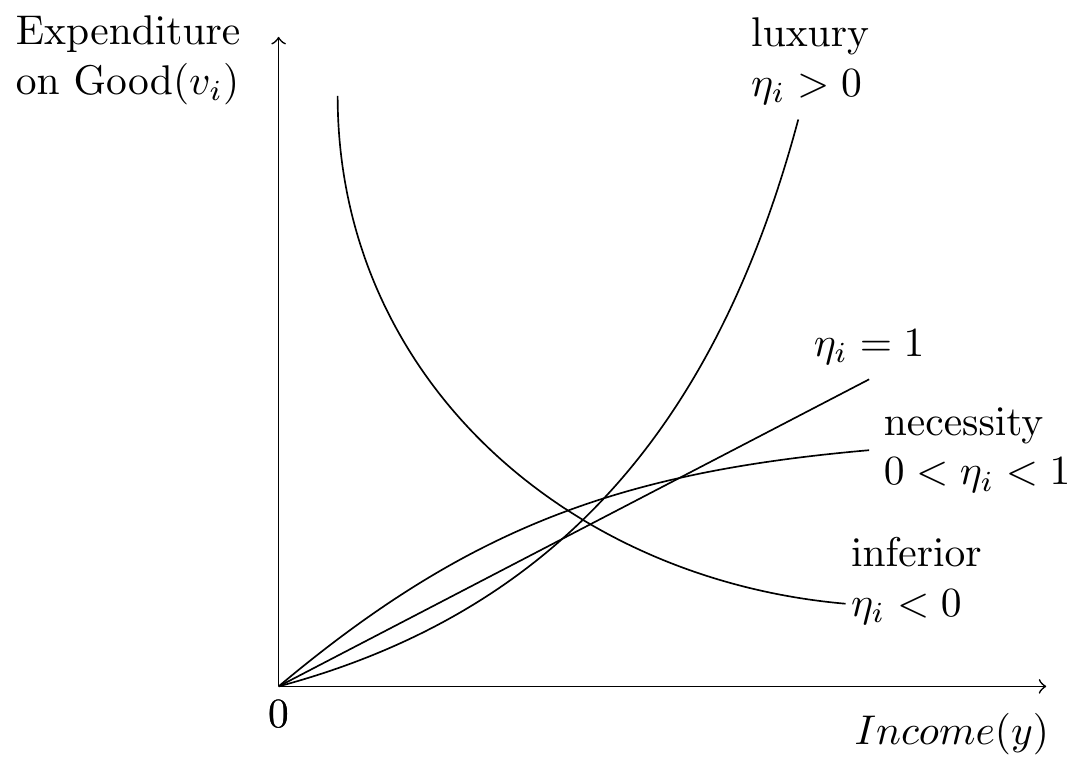
Engle Curve

\begin{tikzpicture}[scale=1]
\draw [->] (0,0) node [below] {0} -- (0,0) -- (6.5,0);
\draw [->] (0,0) node [below] {0} -- (0,0) -- (0,5.5);
\node [align=left, left] at (-0.2,5.3) {Expenditure\\ on Good$(v_i)$};
\node [below] at (5.7,-0.1) {$Income(y)$};
\draw (0,0) to [out=15,in=255] (4.4,4.8);
\node [align=left, above] at (4.5,4.8) {luxury\\ $\eta_i>0$};
\draw (0.5,5) to [out=270,in=175] (4.8,0.7);
\node [align=left, above] at (5.4,0.4) {inferior\\ $\eta_i<0$};
\draw (0,0) to [out=40,in=185] (5,2);
\node [align=left, right] at (5,2) {necessity\\ $0<\eta_i<1$};
\draw (0,0)--(5,2.6);
\node [above] at (5,2.6) {$\eta_i=1$};
\end{tikzpicture}
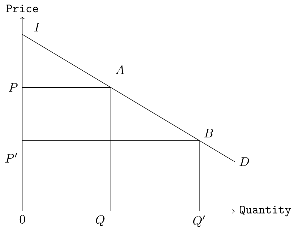
Consumer Surplus

\begin{tikzpicture}[scale=1]
\draw [->] (0,0) node [below] {0} -- (0,0) -- (6,0) node [right] {$\texttt{Quantity}$};
\draw [->] (0,0) node [below] {0} -- (0,0) -- (0,5.5) node [above] {$\texttt{Price}$};
\draw (0,5)--(6,1.4);
\node [right] at (6,1.4) {$D$};
\draw (0,3.5)--(2.5,3.5);
\draw (0,2)--(5,2);
\draw (5,2)--(5,0);
\draw (2.5,0)--(2.5,3.5);
\node [right] at (5,2.2) {$B$};
\node [right] at (2.5,4) {$A$};
\node [right] at (.2,5.2) {$I$};
\node [left] at (0,1.5) {$P'$};
\node [left] at (0,3.5) {$P$};
\node [below] at (2.2,0) {$Q$};
\node [below] at (5,0) {$Q'$};
\end{tikzpicture}
