Advanced Excel
Learning Objectives:
- Add-in
- Analysis Toolpak
- Sorting
- Filtering
- Pivot Table
- Freeze plane
- Charting
- Conditional Statement
Useful tools
Add-in
If you see Analysis Toolpak under the Active Application Add-Ins section, you do not need to do anything. Otherwise, you need to activate it.


If you want to enable Analysis toolpak, go to Options > Add-Ins > Analysis Toolpak. The same goes for Solver.
Analysis Toolpak: Regression
Analysis Toolpak lets you run multiple regressions in Excel.
Analysis Toolpak: Solver
Solver lets you solve linear and nonlinear equations, by optimizing the variables. This is extremely useful when you have a regression with multiple variables that you need to estimate. However, one drawback is that it can give you multiple solutions, so you might get a different answer when you re-run it. To check if you have enabled it, go to Options > Add-Ins > Solver.
However, one drawback of using Solver is that it can have multiple solutions, meaning that the solution changes every time you run it.
We will cover other useful tools such as sorting, filtering, pivot table, freeze plane, split plane, and charting.
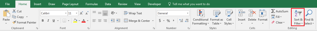
Sorting
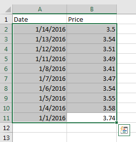
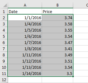
Sometimes, data that you download is in descending order of date, meaning that the most recent data is at the top. If you want to change the dates to be in ascending order(i.e. the latest date is at the bottom), you can use the Sort function in Excel.
First, select your data. This step is necessary. If you have corresponding data, for example, prices that correspond to the dates, you have to select them as well. Otherwise, only the dates will be sorted, and the prices will correspond to the wrong dates.

Filtering
You can also filter data using the Filter option, and this is useful in pinpointing a particular subset of data.
After selecting the Filter function, you will then see a small button on the top right-hand corner of your selected range. Clicking on it will show you the following figure.
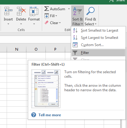

You can then choose how you want to filter the data.
Subtotal
After filtering the data, one natural question is how to calculate summarize the filter data. For example, we want to calculate the sum or average of filter data. For example, we might want to know the sales of product grouped by region. One straightforward way is to produce subtables using SUMIF, COUNTIF or AVERAGEIF.
We employ the function \subtotal(function, range). Where function is an integer where 1 is average and 9 is sum.
Pivot Table
Excel has a one very efficient tools to do subtotal – Pivot table. It is one of the most powerful tools in Excel. It allows you to calculate subtotal easily.
First, prepare your data in a table form with header. As shown in Figure below.

Then go to insert ribbon and then choose pivot table.Then fill in the table range.

Then you can drag variables into four boxes: filters, columns, rows and values.
The basic elements are rows and values. Rows are the groups needed and values are the summary statistics to be calculated such as sum, average, count, standard deviation.
If we want to include grouping for values, then we can put the variable into columns. If we want to include grouping for everything, then it will be in filter.
For example, consider student record data with following columns: year, semester, course, students, assessment (mid-term, assignment or final), and scores. Then row variable can be course, and then values is scores. Then column is assessment. Filter can be year and semester.
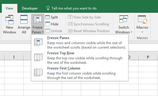
Freeze Plane
When we have large spreadsheet, it is convenient to keep some parts (especially the row or columns headers) while we are scroll away. To do so, we can use freeze plane.
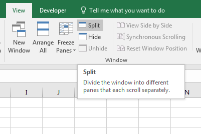
Split Plane
When we have large spreadsheet, we want to compare some parts with another parts. To do so, we can use split plane function.
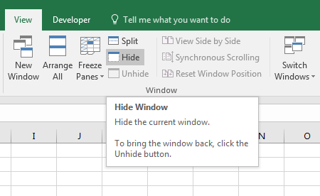
Hide and Unhide
When we have many rows and columns, the screen may be too small to display all. For example, some rows are too bothering to work on. Then we have a row of data we wish to hide. We could do that by simply selecting the row, and pressing the right mouse button, then selecting the hide option.

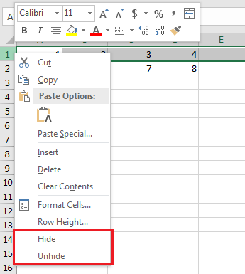
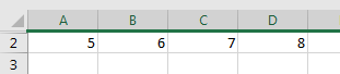
The result would then look like this. You can also unhide row 1 by selecting the unhide option. See Figure \ref{Excel-Hide-Row2}.
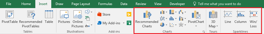
Charting
Excel also allows you to plot charts or graphs easily, to aid in the visualization of data. Simply go to the Insert tab, and there are multiple options available there. See Figure \ref{Excel-Charting}
Conditional
Logical statements are either true or false. Very often, we want to compare two numbers. For example, 2> 1 is true statement but 2 < 1 is false statement.
| Function | Meaning |
|---|---|
> |
Greater than |
< |
Less than |
| = | Equal to |
>= |
Greater than or equal to |
<= |
Less than or equal to |
Conditional function is useful for piece-wise function. One common example is absolute function. It returns the same number if the number is positive but change the number to positive if the given number is negative. The following expression takes the absolute value in the cell A1: =IF(A1>0,A1,-A1).
| Function | Meaning |
|---|---|
| IF (logical, A, B) | It checks whether the logical is true, and returns A value if TRUE, and B if FALSE. |
Here we provide an example of using conditional statement.
For a list of scores: 85, 90, 72, 45…, we want to assign Pass if no less than 50, and Fail otherwise.
| A | B | C | |
|---|---|---|---|
| 1 | Students | Score | Pass? |
| 2 | Peter | 85 | =IF(B2>50,"PASS","FAIL") |
| 3 | John | 94 | |
| 4 | Mart | 72 | |
| 5 | Susan | 45 |
Now we have another example of grading: A for scores no less than 80, B for scores no less than 70, and C otherwise.
| A | B | C | |
|---|---|---|---|
| 1 | Students | Score | Grade |
| 2 | Peter | 85 | =IF(B2>80,"A",IF(B2>70,"B","C")) |
| 3 | John | 94 | |
| 4 | Mart | 72 | |
| 5 | Susan | 45 |
Next example is about the most simplest technical trading rule – simple filter rule. We calculate the price change P(t)/P(t-1) in column C and then for column D we use conditional statement to set Buy=1 when the price change is greater than $1+\delta$ and Buy=0 otherwise.
| A | B | C | D | |
|---|---|---|---|---|
| 1 | Delta | 0.02 | ||
| 2 | Date | P(t) | P(t)/P(t-1) | Buy |
| 3 | 02-May-16 | 10 | ||
| 4 | 03-May-16 | 12 | =C4/C3 |
=IF(C4>1+$B$1,1,0) |
| 5 | 04-May-16 | 11 |
Then we can add sell variable at column D. It is set to 1 when the price change is less than $1-\delta$ and Buy=0 otherwise. Finally, column E is the trading signal, and it is sum of buy and sell.
| A | B | C | D | E | F | |
|---|---|---|---|---|---|---|
| 1 | Delta | 0.02 | ||||
| 2 | Date | P(t) | P(t)/P(t-1) | Buy | Sell | Trade |
| 3 | 02-May-16 | 10 | ||||
| 4 | 03-May-16 | 12 | =C4/C3 |
=IF(C4>1+$B$1,1,0) |
=IF(C4<1-$B$1,-1,0) |
=D4+E4 |
| 5 | 04-May-16 | 11 |
There are some conditional functions: COUNTA only counts non-empty cell, and COUNTBLANK counts blank cell. COUNTIF only counts cells with specific criteria. SUMIF and AVERAGEIF only sum and average over cells with specific criteria.
| Function | Meaning |
|---|---|
| COUNTA(range) | Counts the number of cells in a range that are not empty |
| COUNTBLANK(range) | Counts the number of empty cells in a specified range of cells |
| COUNTIF(range, criteria) | Counts the number of cells within a range that meet the given condition. For example, COUNTIF("A1:B2",">0") counts the number of cells with positive number |
| SUMIF(range, criteria) | Adds the cells specified by a given condition or criteria |
| AVERAGEIF(range, criteria) | Finds average(arithmetic mean) for the cells specified by a given condition or criteria |
Sometimes, we want to combine several logical statements.
| Function | Meaning |
|---|---|
| AND(logical1, logical2) | Returns TRUE if both logicals are TRUE |
| OR(logical1, logical2) | Returns TRUE if any of the logicals are TRUE, and Returns FALSE only if all logicals are FALSE |
| NOT(logical) | Changes FALSE to TRUE, or TRUE to FALSE |
Now we have another example of grading. Grading depends on the sum of test and exam. Similar to the above example, a student will get an A for scores no less than 80, a B for scores no less than 70, and a C otherwise. However, if an A student score more than 60 in final, A+ will be given.
| A | B | C | D | |
|---|---|---|---|---|
| 1 | Student | Test | Exam | Grade |
| 2 | Pert | 30 | 55 | =IF(AND(B2+C2>80,C2>60),"A",IF(B2+C2>80,"A",IF(B2+C2>70,"B","C")) |
| 3 | John | 28 | 62 | |
| 4 | Mary | 22 | 40 | |
| 5 | Susan | 45 | 40==30 |
For technical analysis, we usually use more than one signals. To combine two signals, one common method is to take action when both signals agree. It combines two buy signals (columns A and B) into final signal (column C).
| A | B | C | |
|---|---|---|---|
| 1 | Rule1 | Rule2 | Buy? |
| 2 | 0 | 1 | =IF(AND(A1=1,B1=1),1,0) |
| 3 | 1 | 0 | |
| 4 | 0 | 1 | |
| 5 | 1 | 0 |
More applications
Excel spreadsheet can be used for fundamental analysis, technical analysis and simulation.
Fundamental Analysis
We can construct the spreadsheet of performance ratio analysis from data generated from financial statements of a given year. Vlookup will be useful in this case. We can also use the copy and paste function to replicate the analysis for other years. Relative address will be useful here.
Technical analysis
We can also perform technical analysis in Excel, by setting up our own spreadsheet and incorporating the formula. Examples include Filter rule, Simple Moving Average (SMA),Exponential Moving Average (EMA), Bollinger Band, Moving Average Convergence Divergence (MACD), Relative Strength Index (RSI).
Time Series Analysis
We can also do some basic time series analysis in Excel spreadsheet. Examples include, Gaussian White Noise, Moving Average MA1 model, Autoregressive AR1 model, Random Walk.