Basic Excel
Learning Objectives:
- Why Excel?
- Basic Excel
- Worksheet Functions
What is Excel? Why Excel?
Excel is a spreadsheet program. It is widely used in the industry because they are simple, and also allow you to view data visually.
Since Excel is widely used, it is usually the basic requirement for many jobs.
Here, we will go into the basics of Excel, and how to use them.
Cells
The basic element of spreadsheet is a cell. We often work with multiple cells. Some cells will be data, some cells will be calculation steps and some cells contains results that require calculations.
Another cell in the same sheet
The first thing to learn in excel is how to refer to another cell. There are 2 ways to reference cells:
- A1 method and
- R1C1 method.
The A1 method is more commonly used, since the columns are already labeled with letters, and the rows are labeled by numbers.
However, if your dataset has many columns (more than 26), it might be a good idea to use the R1C1 method.
To calculate the sum of 2 cells A1 and B1, simply type in the equation box:
= A1 + B1.
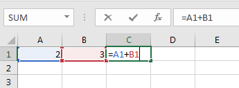
Pressing the Enter key will then give you the following result.
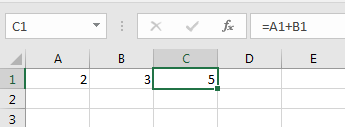
This is assuming that both A1 and B1 contain numerical values. Otherwise, you will get a \#VALUE! Error.
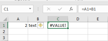
If you place your mouse cursor on the yellow diamond box, it will tell you what error has occurred.
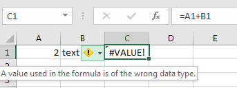
Because A1 contains a numerical value, and B1 contains text, you cannot apply the Sum function, hence Excel raises an error. We then show an example of multiplication as below.
Range, Worksheet and Workbook
We sometimes need to refer to a group of cells for calculation. Range is always rectangular, hence, we just need the top left cell and bottom right cell. For example, A1:B2 implies cells A1, A2, B1, and B2.
To refer to cells in other worksheet in the same workbook (xlsx file), we use the name and exclamation mark. For example, =Sheet1!A1
To refers to cells in the other worksheet in the different workbook, we use squared bracket. For example, =[appl.xlsx]Sheet1!A1 for workbook that is currently open in Excel. Alternatively, ='C:\\document\\[appl.xlsx]'Sheet1!A1 for workbook that is not open.
Copy and Paste: Iteration
Copy and Paste is the most commonly used operation in Excel. It is very powerful tools to perform calculation repetitively. In programming terminology, it is called iteration.
Referencing: Absolute vs. Relative
You can use absolute referencing, or relative referencing. We start by explaining relative referencing.
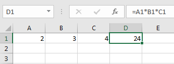
Say I have the following values for columns A, B, and C, and I want to calculate D as their product. If I simply copy D1 and paste it in D2, by default Excel will take it as relative referencing, and D2 = A2*B2*C2 = 210.
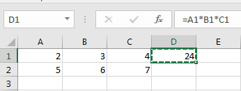

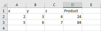
What if I want to reuse the value of A1, say I want D2 = A1*B2*C2? We then use the $ sign to indicate absolute referencing. Placing the $ sign in front of the row or column of the cell will tell Excel to always take that particular row or column even when the formula is copied.
Tips: Pressing F2 will change between relative address and absolute address.


We see that D2=A1*B2*C2 even when we copied the formula from D1. Because of the $ in $A$1, Excel did not use relative referencing for that row/column.
The following example shows how relative address can be used effectively to reduce typing when we create multiplication table. We just need to enter the formula in B2. Then copy and paste the rest of the cells.
| A | B | C | |
|---|---|---|---|
| 1 | x | 1 | 2 |
| 2 | 1 | =$A2*B$1 |
|
| 3 | 2 |
Naming
Usually, we will label our rows and/or columns, to let the user know what kind of data or variables are in the spreadsheet. This is for convenience so that the user can follow what you are doing easily.
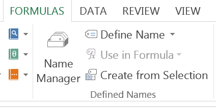
Moreover, we give a name to a cell. In the ribbon, choose FORMULAS tab and then choose to define the name. Then you can refer a cell by its name. This is particularly useful to make your spreadsheet easy to read and understand by other users.
dividend discount model
Let us illustrate the idea of relative address using the dividend discount model(DDM) example. Consider stock which pays out a fixed dividend of $1 per year for the next 10 years. The rate of inflation is going to be constant at 3% per year. We want to find out how much the future dividend payouts are worth in present values.
The discount factor is equal to 1/1.03, which is approximately 0.9709. How do we do this calculation efficiently in Excel? We make use of both relative and absolute referencing.
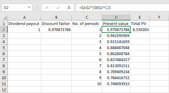
The only thing that changes here is the overall discount factor, which depends on the number of years ahead. Hence we use absolute referencing for the dividend payout amount, and the yearly discount factor, and then multiply the yearly discount factor accordingly with the number of years. Lastly, we sum up the values to get 8.53.
Worksheet Functions
Excel spreadsheet is very convenient because it has a large number of built-in functions that perform calculation without programming. We will learn how to write these functions by yourself in the next class using VBA.
Arithmetic Operators
We first cover some basic arithmetic operators and some basic mathematics functions.
| Function | Meaning |
|---|---|
+ |
Addition |
- |
Substraction |
* |
Multiplication |
/ |
Division |
^ |
Power |
| SQRT() | Square Root |
| ABS() | Absolute number |
Basic Math Functions
| Function | Meaning |
|---|---|
| COUNT(range) | Counts the number of cells in a range that contain numbers |
| SUM(range) | Adds all the numbers in a range of cells |
| PRODUCT(range) | Multiplies all the numbers given as arguments |
| SUMPRODUCT(range1, range2) | Sum of products of the first elements in both ranges, the second elements,…. |
Basic Statistic Functions
| Function | Meaning |
|---|---|
| MIN(range) | Returns the smallest number in a set of values. Ignores logical values and text |
| MAX(range) | Returns the largest number in a set of values. Ignores logical values and text |
| MEDIAN(range) | Returns the median, or the number in the middle of the set of given numbers |
| VAR.P(range) | Calculates population variance |
| VAR.S(range) | Calculates sample variance |
| STDEV.P(range) | Calculate population standard deviation |
| STDEV.S(range) | Calculate sample standard deviation |
The following example shows AVERAGE is used to calculate simple moving average.
| A | B | C | |
|---|---|---|---|
| 1 | n | 5 | |
| 2 | beta | =2/(A1+1) |
|
| 3 | Date | Price | SMA(n) |
| 4 | 02-May-16 | 19 | |
| … | |||
| 7 | 06-May-16 | 30 | =AVERAGE(B3:B7) |
| 8 | 07-May-16 | 56 |
The following example shows AVERAGE and recursive formula is used to calculate exponential moving average. Note that initial EMA is SMA. And the recursive formula is $$EMA_{t}(n) = \beta P_{t}(n) + (1-\beta) EMA_{t-1}(n)$$
where $\beta=2/(n+1)$.
| A | B | C | |
|---|---|---|---|
| 1 | n | 5 | |
| 2 | beta | =2/(A1+1) |
|
| 3 | Date | Price | EMA(n) |
| 4 | 02-May-16 | 19 | |
| … | |||
| 7 | 06-May-16 | 30 | =AVERAGE(B3:B7) |
| 8 | 07-May-16 | 56 | =$B$2*B9+(1-$B$2)*C8 |
Advanced Statistic Functions
| Function | Meaning |
|---|---|
| COVARIANCE.P(range1 ,range2) | Calculate population covariance using data in range 1 and range 2 |
| COVARIANCE.S(range1, range2) | Calculate sample covariance using data in range 1 and range 2 |
| INTERCEPT(yrange,xrange) | Returns the intercept of simple linear regression of y on x |
| SLOPE(yrange, xrange) | Returns the slope of simple linear regression of y on x |
| STEYX(yrange, xrange) | Returns the standard error of simple linear regression of y on x |
| RAND() | Returns a random number greater than or equal to 0 and less than 1, evenly distributed |
| RANDBETWEEN(integer1, integer2) | Returns a random number between integer1 and integer 2 where integer1 is less than integer2 |
| NORM.INV(probability, mean, standard deviation) | Returns the inverse of the normal cumulative distribution at the given probability under the specified mean and standard deviation. |
How to generate normal distribution? We will use a method called inversion. Use RAND to generate uniform distribution and then use NORM.INV is to generate a normal variable.
Lookup
Lookup functions allow you to get data from another table. Two basic lookup functions are VLOOKUP or HLOOKUP. They help to locate particular cells in table. Using MATCH and INDEX together allows us to have a flexible vlookup and hlookup, when we have 2 different types of data.
For example, we could use =INDEX(range1, MATCH(key, range2)).
| Function | Meaning |
|---|---|
| VLOOKUP(key, range, column, FALSE) | Looks for key in the leftmost column of a table (given by the range), and then returns a value in the same row from a column you specify. |
| HLOOKUP(key, range, column, FALSE) | Looks for key in the top row of a table (given by the range) and returns the value in the same column from a row you specify. |
| MATCH(key, range) | This helps you search for a particular value within a dataset. The output returned is the relative position of the value in the dataset, for example, D8. The key is the value that you want to find, and the range is the range of data that you are searching for. |
| INDEX(range, index) | Returns a value or reference of the cell at the intersection of a particular row and column, in a given range. The output will be the content of that particular cell at that index. |
The following example shows how vlookup can be used to merge two tables.
| A | B | C | D | |
|---|---|---|---|---|
| 1 | Stock | Price | Stock | Volume |
| 2 | Apple | 10 | IBM | 10 |
| 3 | IBM | 20 | 20 | |
| 4 | 30 | Apple | 30 | |
| 5 | ||||
| 6 | Stock | Price | Volume | |
| 7 | Apple | =VLOOKUP(A7,$A$1:$B$4,2,FALSE) |
=VLOOKUP(A7,$C$1:$D$4,2,FALSE) |
|
| 8 | IBM | |||
| 9 |
The following example shows how index and match can be used to merge two tables.
| A | B | C | D | |
|---|---|---|---|---|
| 1 | Stock | Price | Stock | Volume |
| 2 | Apple | 10 | IBM | 10 |
| 3 | IBM | 20 | 20 | |
| 4 | 30 | Apple | 30 | |
| 5 | ||||
| 6 | Stock | Price | Volume | |
| 7 | Apple | =INDEX(B2:B4,MATCH(A7, A2:A4,0)) |
=INDEX(D2:D4, MATCH(A7,C2:C4,0)) |
|
| 8 | IBM | |||
| 9 |
Cell Referencing Function
The following cell referencing functions are very useful to make the code clean and tidy. Offset moves the cell reference to another cell or range of cells. Indirect convert text to cell reference and Address convert cell reference to text.
| Function | Meaning |
|---|---|
| OFFSET(cell, row, column,height and width) | Returns a reference to a range that is a given number of rows and columns from a given reference. Cell refers to the reference cell that you are taking reference from. For row, positive values will mean cells downwards from the reference cell, and negative values will mean cells above the reference cell. For column, positive values will mean cells to the right of the reference cell, while negative values will mean cells to the left of the reference cell. |
| INDIRECT(address string) | Returns the reference specified by a text string. One example would be INDIRECT("A1"), which returns the contents of the cell A1. |
| ADDRESS(row, column) | Creates a cell reference as text, given specified row and column numbers. For example, ADDRESS(2, 7) will return $G$2 as output. |
Combination of INDIRECT and ADDRESS is useful if you do not want to type out the address string, or you have very large datasets. We can use INDIRECT(ADDRESS(1,2)).
The following example shows offset can be used to make spreadsheet customization. We consider K-day momentum where K allow the user to input. While OFFSET is rather simple, we need to take care the case when momentum cannot be calculate in the first K days.
| A | B | C | |
|---|---|---|---|
| 1 | K | 5 | |
| 2 | Date | Price | K-Momentum |
| 3 | 02-May-16 | 10 | =IF(COUNT($A$3:A3)>=$B$1+1,B3-OFFSET(B3,-$B$1), "") |
| 4 | 03-May-16 | 9 | |
| 5 | 04-May-16 | 8 |
The following sample shows more advanced use of OFFSET. We consider n-day simple moving average where n allows the user to input. We only start the calculation when on the n-th day.
| A | B | C | |
|---|---|---|---|
| 1 | n | 5 | |
| 2 | Date | Price | SMA(n) |
| 4 | 02-May-16 | 10 | =IF(COUNT($A$3:A3)>=$B$1,average(Offset(B3,0,0,-$B1$)), "") |
| 5 | 03-May-16 | 9 | |
| 6 | 04-May-16 | 8 |
The following sample shows more advanced use of OFFSET. We consider n-day simple moving average where n allows the user to input. We only start the calculation of EMA when on the n-th day. The first EMA is SMA. Then the rest is by the updating recursive formula.
| A | B | C | |
|---|---|---|---|
| 1 | n | 5 | |
| 2 | beta | =2/(A1+1) |
|
| 3 | Date | Price | EMA(n) |
| 4 | 02-May-16 | 19 | =IF(COUNT($A$4:A4)=$B$1,average(Offset(B4,0,0,-$B1$)),IF(COUNT($A$4:A4)>$B$1,=$B$2*B4+(1-$B$2)*C3, "") |
| 5 | 03-May-16 |
Hyperlink
The following function refers the external link. Hyperlink connects to external file or internet address.
| Function | Meaning |
|---|---|
| HYPERLINK(location, text) | Creates a shortcut or jump that opens a document stored on your hard drive, a network server, or on the internet. For location, you could use places on your computer such as Desktop or C:, or use internet address such as http://www.google.com. The text will be shown as a hyperlink, for example, you could put Click to open Google search'. |
Text Function
The following shows some basic text functions. Len is to find the length. Trim and Clean is to clean up the text. Concatenate is to combine text.
| Function | Meaning |
|---|---|
| LEN(text) | Short form for length. Returns the number of characters in a text string. For example, LEN(apple) returns 5. |
| TRIM(text) | Removes all spaces from a text string except for single spaces between words. |
| CLEAN(text) | Removes all nonprintable characters from text. |
| CONCATENATE(text1, text2, …) | Joins all text strings into one text string. For example, CONCATENATE("I am", "a boy", ...) returns I ama boy. Note that space is not automatically added between text. |
There are some advanced text functions: Left, Right and Mid extract part of text. Find and Search are to look for string and Substitute is to replace text.
| Function | Meaning |
|---|---|
| LEFT(text, number) | Returns the specified number of characters from the left of the text string. For example, LEFT("testing", 2) will return you te. |
| RIGHT (text, number) | Returns the specified number of characters from the right of the text string. For example, RIGHT("testing", 2) will return you ng. |
| MID (text, start position, number) | Returns the specified number of characters from the start position of the text string. For example, MID("testing", 3,2) will return you st |
| FIND(text, target) | Returns the starting position of one text string within the target text string. For example, FIND("apple", "I like apple") returns 8. Note that FIND is case-sensitive, meaning that upper-case letters are not the same as lower-case letters. For example, FIND("APPLE", "I like apple") returns an error. |
| SEARCH(text, target) | Same as FIND but not case-sensitive. For example For example, SEARCH("APPLE", "I like apple") returns 8 |
| SUBSTITUTE(target, new text, old text) | Replaces existing text with new text in a text string. For example, SUBSTITUTE("I like apple", "apple", "banana") returns I like banana. |