Statistical Analysis

We first review some basic function of statistics: central tendency and dispersion before going into regression analysis.

Learning objectives:

summary statics
generate random numbers
estimate OLS
estimate time series models (ARIMA using arima, GARCH using rugarch, VAR using vars)
estimate panel data (plm package)
Simulation on random walk model and Roll model

Basic Statistics

Central Tendency

x <- 1:40
mean(x)

## [1] 20.5

median(x)

## [1] 20.5

summary(x)  #Five-number summary

##    Min. 1st Qu.  Median    Mean 3rd Qu.    Max. 
##    1.00   10.75   20.50   20.50   30.25   40.00

Dispersion

range(x)     #Get minimum and maximum

## [1]  1 40

IQR(x)       #Inter-quartile range

## [1] 19.5

var(x)       #variance

## [1] 136.6667

sd(x)        #Standard deviation

## [1] 11.69045

Random number

To generate random integers, we use the function sample().

We first generate 8 random integers between 2 and 10 without replacement:

sample(2:10,8, replace=F)

## [1]  4  5  6  9 10  2  3  8

The next one generate 7 integers between 2 and 10 with replacement:

sample(2:10,7, replace=T)

## [1] 10  6  5  5  2  6  6

In general, the sample() function can also be applied to extract random element from a vector.

namelist<-c("Mary", "Peter", "John", "Susan")
sample(namelist,2)  # sample from this list

## [1] "Susan" "Mary"

To generate random decimal numbers, we use runif to get random uniform distribution. The following generates 2 random decimal numbers between 4.6 and 7.8:

runif(2, 4.6, 7.8)

## [1] 7.169279 4.839000

To generate normal distribution, we use rnorm(). The following generate 4 random number that follows the normal distribution with mean being 0 and standard deviation being 1.

x <- rnorm(4, mean=0, sd=1) # standard nromal
x

## [1]  1.8976780 -0.2299555  1.2559706 -0.9824391

Regression

We will be using the following data to show the regression. Note that we need to use dataframe.

x <- c(1,2,3,5,6,7,10,12,13)
y <- c(1,4,5,6,7,8,9,10,15)
z <- c(2,3,7,8,9,12,8,7,6)
df <-data.frame(x=x,y=y,z=z)

Simple linear regression

The following code shows simple linear regression. The syntax is lm(y~x, dataframe).

SLR <-lm(y~x,df)
summary(SLR)

## 
## Call:
## lm(formula = y ~ x, data = df)
## 
## Residuals:
##     Min      1Q  Median      3Q     Max 
## -1.9660 -1.2234  0.2618  0.7470  2.1627 
## 
## Coefficients:
##             Estimate Std. Error t value Pr(>|t|)    
## (Intercept)   1.5104     0.8756   1.725 0.128193    
## x             0.8713     0.1134   7.686 0.000118 ***
## ---
## Signif. codes:  0 '***' 0.001 '**' 0.01 '*' 0.05 '.' 0.1 ' ' 1
## 
## Residual standard error: 1.389 on 7 degrees of freedom
## Multiple R-squared:  0.8941, Adjusted R-squared:  0.8789 
## F-statistic: 59.08 on 1 and 7 DF,  p-value: 0.0001175

Muliple linear regression

The following code shows multiple regression. The syntax is lm(y~x+z, dataframe).

MLR <-lm(y~x + z,df)
summary(MLR)

## 
## Call:
## lm(formula = y ~ x + z, data = df)
## 
## Residuals:
##     Min      1Q  Median      3Q     Max 
## -1.8920 -1.2104  0.1329  0.8179  2.3030 
## 
## Coefficients:
##             Estimate Std. Error t value Pr(>|t|)    
## (Intercept)  1.25034    1.34526   0.929 0.388522    
## x            0.85666    0.13321   6.431 0.000668 ***
## z            0.05167    0.19124   0.270 0.796060    
## ---
## Signif. codes:  0 '***' 0.001 '**' 0.01 '*' 0.05 '.' 0.1 ' ' 1
## 
## Residual standard error: 1.492 on 6 degrees of freedom
## Multiple R-squared:  0.8953, Adjusted R-squared:  0.8605 
## F-statistic: 25.67 on 2 and 6 DF,  p-value: 0.001146

Interaction terms

The following code shows multiple regression with interaction term. The syntax is lm(y~x+z+x:z, dataframe).

MLRDummy <- lm(y ~ x + z + x:z, df)
summary(MLRDummy)

## 
## Call:
## lm(formula = y ~ x + z + x:z, data = df)
## 
## Residuals:
##       1       2       3       4       5       6       7       8       9 
## -0.3080  0.9573 -0.3143 -0.7246 -0.1773  1.1230 -0.5891 -1.6242  1.6572 
## 
## Coefficients:
##             Estimate Std. Error t value Pr(>|t|)  
## (Intercept) -1.33212    1.96748  -0.677   0.5284  
## x            1.59845    0.46581   3.432   0.0186 *
## z            0.64902    0.40027   1.621   0.1658  
## x:z         -0.12819    0.07789  -1.646   0.1607  
## ---
## Signif. codes:  0 '***' 0.001 '**' 0.01 '*' 0.05 '.' 0.1 ' ' 1
## 
## Residual standard error: 1.316 on 5 degrees of freedom
## Multiple R-squared:  0.9321, Adjusted R-squared:  0.8914 
## F-statistic: 22.89 on 3 and 5 DF,  p-value: 0.002386

Robust standard error

To have robust variance-covariance matrix, we have to use package sandwich to get the appropriate error term. Then we do the estimate through the package lmtest

First we install and load the packages.

install.packages(c("sandwich","lmtest"))
library(sandwich)
library(lmtest)

Then we need to create the variance and covariance matrix: using the vcovHC().

To match the stata robust command result, we use HC1(). Then we perform coeftest based on specified variance-covariance matrix.

MLR <- lm(y ~ x + z, df)
coeftest(MLR, vcov = vcovHC(MLR, "HC1"))

## 
## t test of coefficients:
## 
##             Estimate Std. Error t value Pr(>|t|)   
## (Intercept) 1.250343   1.117886  1.1185 0.306129   
## x           0.856663   0.194468  4.4052 0.004543 **
## z           0.051674   0.167447  0.3086 0.768062   
## ---
## Signif. codes:  0 '***' 0.001 '**' 0.01 '*' 0.05 '.' 0.1 ' ' 1

Time Series Analysis

Time Series data

Function ts convert any vector into time series data.

price <- c(2,3,7,8,9,12,8,7)
price <- ts(price)
price

## Time Series:
## Start = 1 
## End = 8 
## Frequency = 1 
## [1]  2  3  7  8  9 12  8  7

We first define a time series (ts) object for the estimation. Note that ts is similar to xts but without date and time.

df <- data.frame(a = c(3,4,5),
                 b = c(1,2,4),
                 d = c(1,2,3))
df <- ts(df)
df

## Time Series:
## Start = 1 
## End = 3 
## Frequency = 1 
##   a b d
## 1 3 1 1
## 2 4 2 2
## 3 5 4 3

Extensible Time Series Data

To handle high frequency data (with minute and second), we need the package xts. The package allows you to define Extendible Time Series (xts) object.

The following code installs and loads the xts package.

install.packages("xts")
library(xts)

Consider the following data for our extendible time series

date <- c("2007-01-03","2007-01-04",
          "2007-01-05","2007-01-06",
          "2007-01-07","2007-01-08",
          "2007-01-09","2007-01-10")
time <- c("08:00:01","09:00:01",
          "11:00:01","13:00:01",
          "14:00:01","15:00:01",
          "15:10:01","15:20:03")
price <- c(2,3,7,8,9,12,8,7)

Now we are ready to define xts object. The code as.POSIXct() convert strings into date format with minutes and seconds.

df <-data.frame(date=date, time=time, price=price)
df$datetime <-paste(df$date, df$time)
df$datetime <-as.POSIXct(df$datetime,
                         format="%Y-%m-%d %H:%M:%S")
df <- xts(df,order.by=df$datetime)

For conversion with dates only, we use POSIXlt() instead of POSIXct().

df <-data.frame(date=date, price=price)
df$date <- as.POSIXct(df$date,format="%Y-%m-%d")
df$price <-as.numeric(df$price)
price <-xts(df[,-1],order.by=df$date)

ARMA

Autoregressive moving average model can be estimated using the arima() function.

The following code estimates an AR(1) model:

price <- c(2,3,7,8,9,12,8,7)
AR1 <- arima(price,c(1,0,0))  
AR1

## 
## Call:
## arima(x = price, order = c(1, 0, 0))
## 
## Coefficients:
##          ar1  intercept
##       0.6661     6.1682
## s.e.  0.2680     2.1059
## 
## sigma^2 estimated as 5.33:  log likelihood = -18.34,  aic = 42.68

The following code estimates an AR(2) model:

AR2 <- arima(price,c(2,0,0))  
AR2

## 
## Call:
## arima(x = price, order = c(2, 0, 0))
## 
## Coefficients:
##          ar1      ar2  intercept
##       0.8301  -0.3026     6.5911
## s.e.  0.3357   0.3638     1.7241
## 
## sigma^2 estimated as 4.831:  log likelihood = -18.01,  aic = 44.02

The following code estimates an MA(1) model:

MA1 <- arima(price,c(0,0,1))  
MA1

## 
## Call:
## arima(x = price, order = c(0, 0, 1))
## 
## Coefficients:
##          ma1  intercept
##       0.7945     6.8862
## s.e.  0.4393     1.3412
## 
## sigma^2 estimated as 4.936:  log likelihood = -18.23,  aic = 42.46

The following code estimates an MA(2) model:

MA2 <- arima(price,c(0,0,2)) 
MA2

## 
## Call:
## arima(x = price, order = c(0, 0, 2))
## 
## Coefficients:
##          ma1     ma2  intercept
##       0.8292  0.1459     6.8262
## s.e.  0.3915  0.3245     1.4677
## 
## sigma^2 estimated as 4.945:  log likelihood = -18.14,  aic = 44.28

The following code estimates an ARMA(1,1) model:

ARMA11 <- arima(price,c(1,0,1))
ARMA11

## 
## Call:
## arima(x = price, order = c(1, 0, 1))
## 
## Coefficients:
##          ar1     ma1  intercept
##       0.3551  0.4889     6.6417
## s.e.  0.7701  0.9088     1.8799
## 
## sigma^2 estimated as 4.911:  log likelihood = -18.08,  aic = 44.16

Sometimes, we just want to keep the coefficient.

coef(ARMA11) #Get coefficient

##       ar1       ma1 intercept 
## 0.3551015 0.4889285 6.6417184

The following code shows the plot of residuals.

plot.ts(ARMA11$residuals)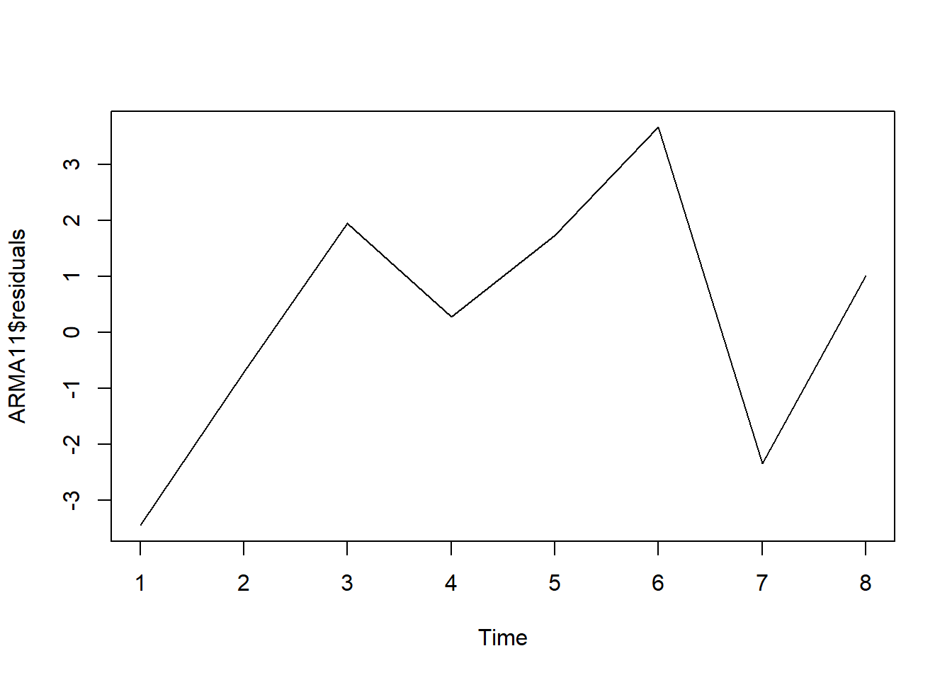

R has a convenient function to autofit() the parameter of ARIMA model. This requires the forecast package. The following code installs and loads the forecast package:

install.packages("forecast") 
library(forecast)

Now we are ready to find the best ARIMA model.

autoarma <-auto.arima (price) 
autoarma

## Series: price 
## ARIMA(0,1,0) 
## 
## sigma^2 estimated as 6.429:  log likelihood=-16.45
## AIC=34.89   AICc=35.69   BIC=34.84

One important function of time series model is forecasting. The following code gives the two-step ahead forecast:

theForecast <-predict(ARMA11,
                      n.ahead=2,
                      se.fit=TRUE)

The following shows the forecast plot.

plot.ts(theForecast$pred) #visualize the forecast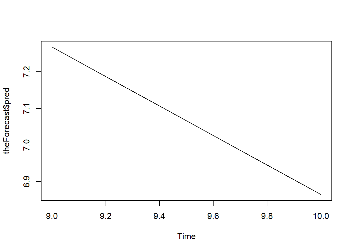

GARCH

To estimate ARCH and GARCH model, we need to install and load package rugarch.

install.packages("rugarch")
library(rugarch)

We will estimate GARCH(1,1) with ARMA(1,1) on generate random number

a <- runif(1000, min=0, max=100) #random number

Spec <-ugarchspec(
  variance.model=list(model="sGARCH",
                      garchOrder=c(1,1)),
  mean.model=list(armaOrder=c(1,1)),
  distribution.model="std") 
Garch <- ugarchfit(spec=Spec, data=a)
Garch

## 
## *---------------------------------*
## *          GARCH Model Fit        *
## *---------------------------------*
## 
## Conditional Variance Dynamics    
## -----------------------------------
## GARCH Model  : sGARCH(1,1)
## Mean Model   : ARFIMA(1,0,1)
## Distribution : std 
## 
## Optimal Parameters
## ------------------------------------
##         Estimate  Std. Error     t value Pr(>|t|)
## mu      48.87905    0.936035  5.2219e+01 0.000000
## ar1      0.29967    1.364823  2.1957e-01 0.826209
## ma1     -0.28485    1.371091 -2.0775e-01 0.835422
## omega    0.98567    3.255287  3.0279e-01 0.762050
## alpha1   0.00000    0.004008  3.6000e-05 0.999971
## beta1    0.99881    0.000064  1.5644e+04 0.000000
## shape   99.99992   39.755740  2.5154e+00 0.011891
## 
## Robust Standard Errors:
##         Estimate  Std. Error     t value Pr(>|t|)
## mu      48.87905    0.920402  5.3106e+01  0.00000
## ar1      0.29967    1.016028  2.9494e-01  0.76804
## ma1     -0.28485    1.018161 -2.7977e-01  0.77966
## omega    0.98567    1.645363  5.9906e-01  0.54913
## alpha1   0.00000    0.002043  7.2000e-05  0.99994
## beta1    0.99881    0.000027  3.6899e+04  0.00000
## shape   99.99992    3.800341  2.6313e+01  0.00000
## 
## LogLikelihood : -4782.165 
## 
## Information Criteria
## ------------------------------------
##                    
## Akaike       9.5783
## Bayes        9.6127
## Shibata      9.5782
## Hannan-Quinn 9.5914
## 
## Weighted Ljung-Box Test on Standardized Residuals
## ------------------------------------
##                         statistic p-value
## Lag[1]                  0.0006312   0.980
## Lag[2*(p+q)+(p+q)-1][5] 0.6316728   1.000
## Lag[4*(p+q)+(p+q)-1][9] 1.7373604   0.993
## d.o.f=2
## H0 : No serial correlation
## 
## Weighted Ljung-Box Test on Standardized Squared Residuals
## ------------------------------------
##                         statistic p-value
## Lag[1]                      3.224 0.07255
## Lag[2*(p+q)+(p+q)-1][5]     3.697 0.29441
## Lag[4*(p+q)+(p+q)-1][9]     5.372 0.37683
## d.o.f=2
## 
## Weighted ARCH LM Tests
## ------------------------------------
##             Statistic Shape Scale P-Value
## ARCH Lag[3]    0.3156 0.500 2.000  0.5742
## ARCH Lag[5]    1.0253 1.440 1.667  0.7254
## ARCH Lag[7]    2.2713 2.315 1.543  0.6600
## 
## Nyblom stability test
## ------------------------------------
## Joint Statistic:  199.444
## Individual Statistics:               
## mu      0.35980
## ar1     0.87529
## ma1     0.87357
## omega   0.04945
## alpha1  0.04962
## beta1   0.04946
## shape  44.27729
## 
## Asymptotic Critical Values (10% 5% 1%)
## Joint Statistic:          1.69 1.9 2.35
## Individual Statistic:     0.35 0.47 0.75
## 
## Sign Bias Test
## ------------------------------------
##                    t-value   prob sig
## Sign Bias           0.9204 0.3576    
## Negative Sign Bias  1.8706 0.0617   *
## Positive Sign Bias  0.3632 0.7165    
## Joint Effect        3.6361 0.3035    
## 
## 
## Adjusted Pearson Goodness-of-Fit Test:
## ------------------------------------
##   group statistic p-value(g-1)
## 1    20     202.1    1.313e-32
## 2    30     226.2    1.980e-32
## 3    40     248.6    2.462e-32
## 4    50     310.7    9.965e-40
## 
## 
## Elapsed time : 0.560498

To obtain specific result of the GARCH model, we use the following code:

coefficient <-coef(Garch)
volatility <- sigma(Garch)
long.run.variance <- uncvariance(Garch)

VAR

The following data will be used to estimate VAR model.

a<- c(3.1,3.4,5.6,7.5,5,6,6,7.5,4.5,
      6.7,9,10,8.9,7.2,7.5,6.8,9.1)
b <- c(3.2,3.3,4.6,8.5,6,6.2,5.9,7.3,
       4,7.2,3,12,9,6.5,5,6,7.5)
d <-c(4,6.2,5.3,3.6,7.5,6,6.2,6.9,
      8.2,4,4.2,5,11,3,2.5,3,6)
df <-data.frame(a,b,d)

To estimate a VAR model, we need to install and load vars packages.

install.packages("vars")
library(vars)

The following code estimates the VAR(2) model.

abvar<-VAR(df,p=2) #run VAR(2)
coef(abvar)        #coefficient estiamte of VAR

## $a
##          Estimate Std. Error    t value  Pr(>|t|)
## a.l1   0.59366615  0.3776796  1.5718776 0.1546224
## b.l1  -0.53728016  0.3153665 -1.7036692 0.1268463
## d.l1   0.06427631  0.2620526  0.2452802 0.8124144
## a.l2   0.59478214  0.4406631  1.3497434 0.2140455
## b.l2  -0.49271501  0.3681374 -1.3383999 0.2175550
## d.l2   0.13247171  0.2139979  0.6190328 0.5531098
## const  4.55502873  2.5585550  1.7803130 0.1128965
## 
## $b
##          Estimate Std. Error    t value   Pr(>|t|)
## a.l1   1.03577283  0.4390665  2.3590341 0.04602757
## b.l1  -0.98047999  0.3666252 -2.6743391 0.02817211
## d.l1   0.43849071  0.3046458  1.4393458 0.18800763
## a.l2   0.77048414  0.5122871  1.5040084 0.17098968
## b.l2  -0.74120465  0.4279733 -1.7318948 0.12153171
## d.l2  -0.08577585  0.2487804 -0.3447853 0.73914487
## const  3.30736245  2.9744145  1.1119373 0.29846082
## 
## $d
##          Estimate Std. Error    t value  Pr(>|t|)
## a.l1   0.09567126  0.4508959  0.2121804 0.8372726
## b.l1   0.37908977  0.3765028  1.0068710 0.3434765
## d.l1   0.26703079  0.3128536  0.8535327 0.4181858
## a.l2   0.23097179  0.5260892  0.4390354 0.6722522
## b.l2  -0.67987321  0.4395038 -1.5469110 0.1604714
## d.l2  -0.18657598  0.2554831 -0.7302869 0.4860477
## const  4.67527066  3.0545515  1.5305915 0.1644018

summary(abvar)     #summary of VAR

## 
## VAR Estimation Results:
## ========================= 
## Endogenous variables: a, b, d 
## Deterministic variables: const 
## Sample size: 15 
## Log Likelihood: -71.865 
## Roots of the characteristic polynomial:
## 0.8034 0.8034 0.6583 0.6583 0.4639 0.4639
## Call:
## VAR(y = df, p = 2)
## 
## 
## Estimation results for equation a: 
## ================================== 
## a = a.l1 + b.l1 + d.l1 + a.l2 + b.l2 + d.l2 + const 
## 
##       Estimate Std. Error t value Pr(>|t|)
## a.l1   0.59367    0.37768   1.572    0.155
## b.l1  -0.53728    0.31537  -1.704    0.127
## d.l1   0.06428    0.26205   0.245    0.812
## a.l2   0.59478    0.44066   1.350    0.214
## b.l2  -0.49272    0.36814  -1.338    0.218
## d.l2   0.13247    0.21400   0.619    0.553
## const  4.55503    2.55856   1.780    0.113
## 
## 
## Residual standard error: 1.552 on 8 degrees of freedom
## Multiple R-Squared: 0.4615,  Adjusted R-squared: 0.0576 
## F-statistic: 1.143 on 6 and 8 DF,  p-value: 0.4184 
## 
## 
## Estimation results for equation b: 
## ================================== 
## b = a.l1 + b.l1 + d.l1 + a.l2 + b.l2 + d.l2 + const 
## 
##       Estimate Std. Error t value Pr(>|t|)  
## a.l1   1.03577    0.43907   2.359   0.0460 *
## b.l1  -0.98048    0.36663  -2.674   0.0282 *
## d.l1   0.43849    0.30465   1.439   0.1880  
## a.l2   0.77048    0.51229   1.504   0.1710  
## b.l2  -0.74120    0.42797  -1.732   0.1215  
## d.l2  -0.08578    0.24878  -0.345   0.7391  
## const  3.30736    2.97441   1.112   0.2985  
## ---
## Signif. codes:  0 '***' 0.001 '**' 0.01 '*' 0.05 '.' 0.1 ' ' 1
## 
## 
## Residual standard error: 1.805 on 8 degrees of freedom
## Multiple R-Squared: 0.616,   Adjusted R-squared: 0.328 
## F-statistic: 2.139 on 6 and 8 DF,  p-value: 0.1578 
## 
## 
## Estimation results for equation d: 
## ================================== 
## d = a.l1 + b.l1 + d.l1 + a.l2 + b.l2 + d.l2 + const 
## 
##       Estimate Std. Error t value Pr(>|t|)
## a.l1   0.09567    0.45090   0.212    0.837
## b.l1   0.37909    0.37650   1.007    0.343
## d.l1   0.26703    0.31285   0.854    0.418
## a.l2   0.23097    0.52609   0.439    0.672
## b.l2  -0.67987    0.43950  -1.547    0.160
## d.l2  -0.18658    0.25548  -0.730    0.486
## const  4.67527    3.05455   1.531    0.164
## 
## 
## Residual standard error: 1.853 on 8 degrees of freedom
## Multiple R-Squared: 0.6278,  Adjusted R-squared: 0.3487 
## F-statistic: 2.249 on 6 and 8 DF,  p-value: 0.143 
## 
## 
## 
## Covariance matrix of residuals:
##         a      b       d
## a  2.4097 0.7713 -1.0454
## b  0.7713 3.2566  0.6701
## d -1.0454 0.6701  3.4345
## 
## Correlation matrix of residuals:
##         a      b       d
## a  1.0000 0.2753 -0.3634
## b  0.2753 1.0000  0.2004
## d -0.3634 0.2004  1.0000

To generate coefficient plot, we need to install and load coefplot package:

install.packages("coefplot")
library(coefplot)

The following code generates the coefficient plot for the VAR model:

coefplot(abvar$varresult$a)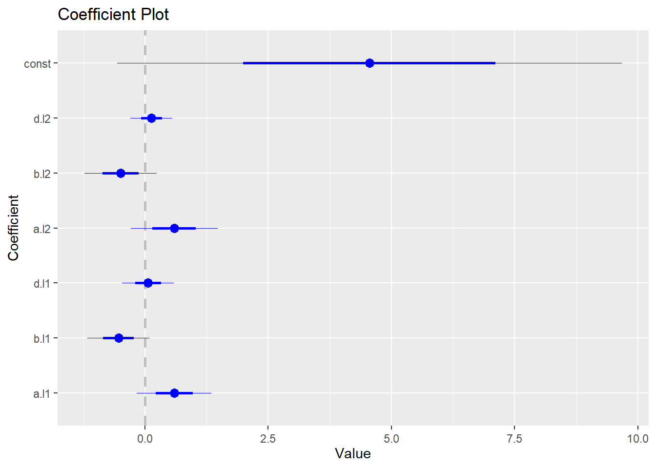

coefplot(abvar$varresult$b)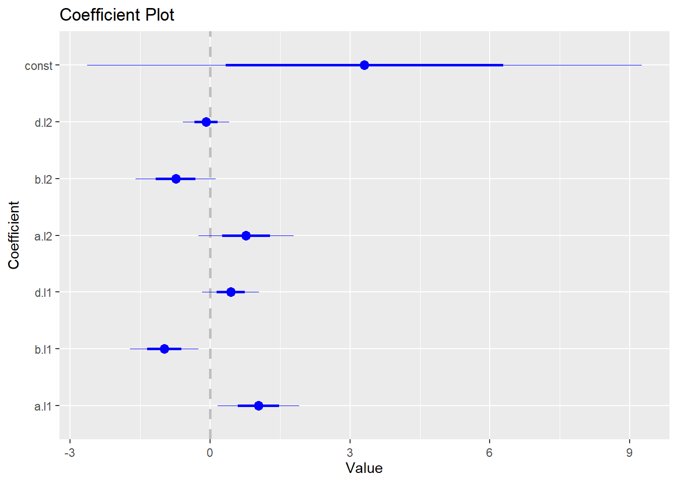

coefplot(abvar$varresult$d)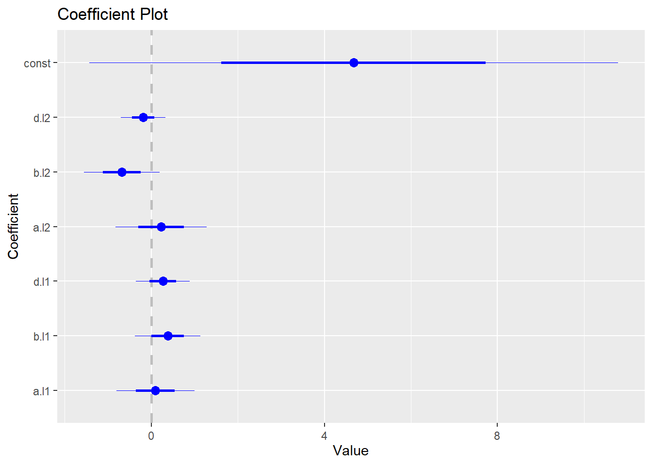

Panel Data

To estimate panel data model, we need to install and load package plm.

install.packages("plm")
library(plm)

We have the following panel data

time <- c(1,2,1,2,1,2,1,2,1,2,1,2)
firm <-c(1,1,2,2,3,3,4,4,5,5,6,6)
x <- c(1, 2, 4, 3, 5, 4, 2, 5,5,6,7,8)
y <- c(2, 3, 5, 4, 3, 2, 4, 7,7,8,5,7)
p.df <- data.frame(time, firm, x, y)
p.df <- pdata.frame(p.df, index = c("firm", "time"), drop.index = F, row.names = T)

Clustering

We first estimate the model based on pooled OLS.

pooled.plm <- plm(formula=y~x, data=p.df, model="pooling")

Then we calculate the variance-covariance matrix to be clustered by group.

coeftest(pooled.plm, vcov=vcovHC(pooled.plm, 
                                 type="sss", 
                                 cluster="group"))

## 
## t test of coefficients:
## 
##             Estimate Std. Error t value Pr(>|t|)   
## (Intercept)  1.81164    0.68521  2.6439 0.024568 * 
## x            0.67808    0.17151  3.9536 0.002715 **
## ---
## Signif. codes:  0 '***' 0.001 '**' 0.01 '*' 0.05 '.' 0.1 ' ' 1

Then we calculate the variance-covariance matrix to be clustered by time.

coeftest(pooled.plm, vcov=vcovHC(pooled.plm, 
                                 type="sss", 
                                 cluster="time"))

## 
## t test of coefficients:
## 
##             Estimate Std. Error t value Pr(>|t|)   
## (Intercept)  1.81164    0.71388  2.5377 0.029478 * 
## x            0.67808    0.21088  3.2154 0.009246 **
## ---
## Signif. codes:  0 '***' 0.001 '**' 0.01 '*' 0.05 '.' 0.1 ' ' 1

Two-way clustering of both time and group:

coeftest(pooled.plm, vcov=vcovDC(pooled.plm, 
                                 type="sss"))

## 
## t test of coefficients:
## 
##             Estimate Std. Error t value Pr(>|t|)  
## (Intercept)  1.81164    0.81130  2.2330  0.04959 *
## x            0.67808    0.22838  2.9691  0.01407 *
## ---
## Signif. codes:  0 '***' 0.001 '**' 0.01 '*' 0.05 '.' 0.1 ' ' 1

Fixed Effect Model

We first estimate the model based on pooled OLS.

fe.plm <- plm(formula=y~x, data=p.df, model="within")

Then we calculate the variance-covariance matrix to be clustered by group.

coeftest(fe.plm, vcov=vcovHC(fe.plm, 
                             type="sss",
                             cluster="group"))

## 
## t test of coefficients:
## 
##   Estimate Std. Error t value  Pr(>|t|)    
## x 1.071429   0.089074  12.028 7.008e-05 ***
## ---
## Signif. codes:  0 '***' 0.001 '**' 0.01 '*' 0.05 '.' 0.1 ' ' 1

Then we calculate the variance-covariance matrix to be clustered by time.

coeftest(fe.plm, vcov=vcovHC(fe.plm, 
                             type="sss", 
                             cluster="time"))

## 
## t test of coefficients:
## 
##     Estimate Std. Error    t value  Pr(>|t|)    
## x 1.0714e+00 4.6089e-10 2324719242 < 2.2e-16 ***
## ---
## Signif. codes:  0 '***' 0.001 '**' 0.01 '*' 0.05 '.' 0.1 ' ' 1

Simulation

We will consider two different simulations:

random walk model, and
Roll model of security price.

Random Walk

We first construct a random walk function that simulates random walk model. It takes the number of period (N), initial value (x0), drift (mu), and variance. The function use rnorm() to generate random normal variable, and then use cumsum() to get the random walk. Note that the whole function is based on vector operation, instead of looping over time.

RW <- function(N, x0, mu, variance) {
  z<-cumsum(rnorm(n=N, mean=0, 
                  sd=sqrt(variance)))
  t<-1:N
  x<-x0+t*mu+z
  return(x)
  }
# mu is the drift

P1<-RW(100,10,0,0.0004)
P2<-RW(100,10,0,0.0004)
plot(P1, main="Random Walk without Drift", 
     xlab="t",ylab="Price", ylim=c(9.7,10.3),
     typ='l', col="red")
par(new=T)  #to draw in the same plot
plot(P2, main="Random Walk without Drift", 
     xlab="t",ylab="Price", ylim=c(9.7,10.3),
     typ='l', col="blue")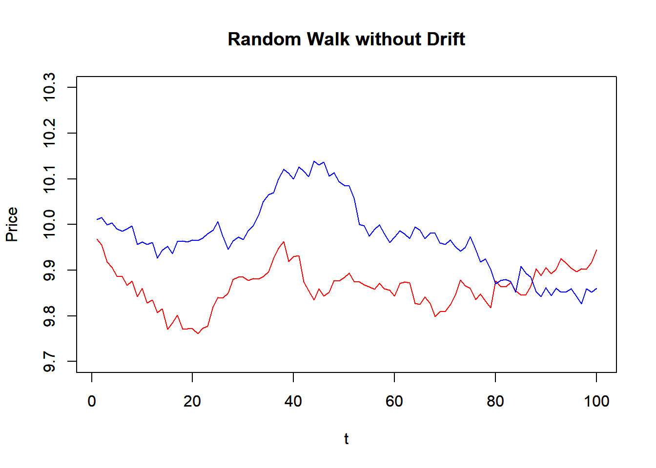

par(new=F)

Roll Model

To simulate the Roll model, we first simulate the price series and simulated trade prices. We calculate the first difference of the price and then we can estimate the first and the second orders of autocovariances. Then we can compare the true trading cost with the estimate one.

require(zoo)

trial <-1000  #Number of trial

cost <-c() #cost each trial
sd <-c()   #sd each trial

true.cost = 2
true.sd = 1

time = 1:trial

for (i in 1:trial) {
  
  #Simulated Price Series
  epsilon = rnorm(time,sd=true.sd)
  prices = cumsum(epsilon)
  m_t = zoo(prices)
  a_t = m_t + true.cost
  b_t = m_t - true.cost
  
  #simulated trade prices 
  q_t = sign(rnorm(time))
  p_t = m_t + (true.cost * q_t)
  
  #1st difference of prices
  delta_p <- p_t-lag(p_t)  
  #omit n.a. entry
  delta_p <- na.omit(delta_p) 

  gamma_0 <- var(delta_p)
  gamma_1 <- cov(delta_p[1:length(delta_p)-1], 
                 delta_p[2:length(delta_p)])
  sigma_2 <- gamma_0 + 2 * gamma_1
  
  if(gamma_1 > 0){
    print("Error: Positive Autocovariance!")
  } else {
    cost <- append(cost,sqrt(-1*gamma_1))
    sd <-append(sd,sigma_2)
  }
}

# Stimulated Cost Plot

plot(cost)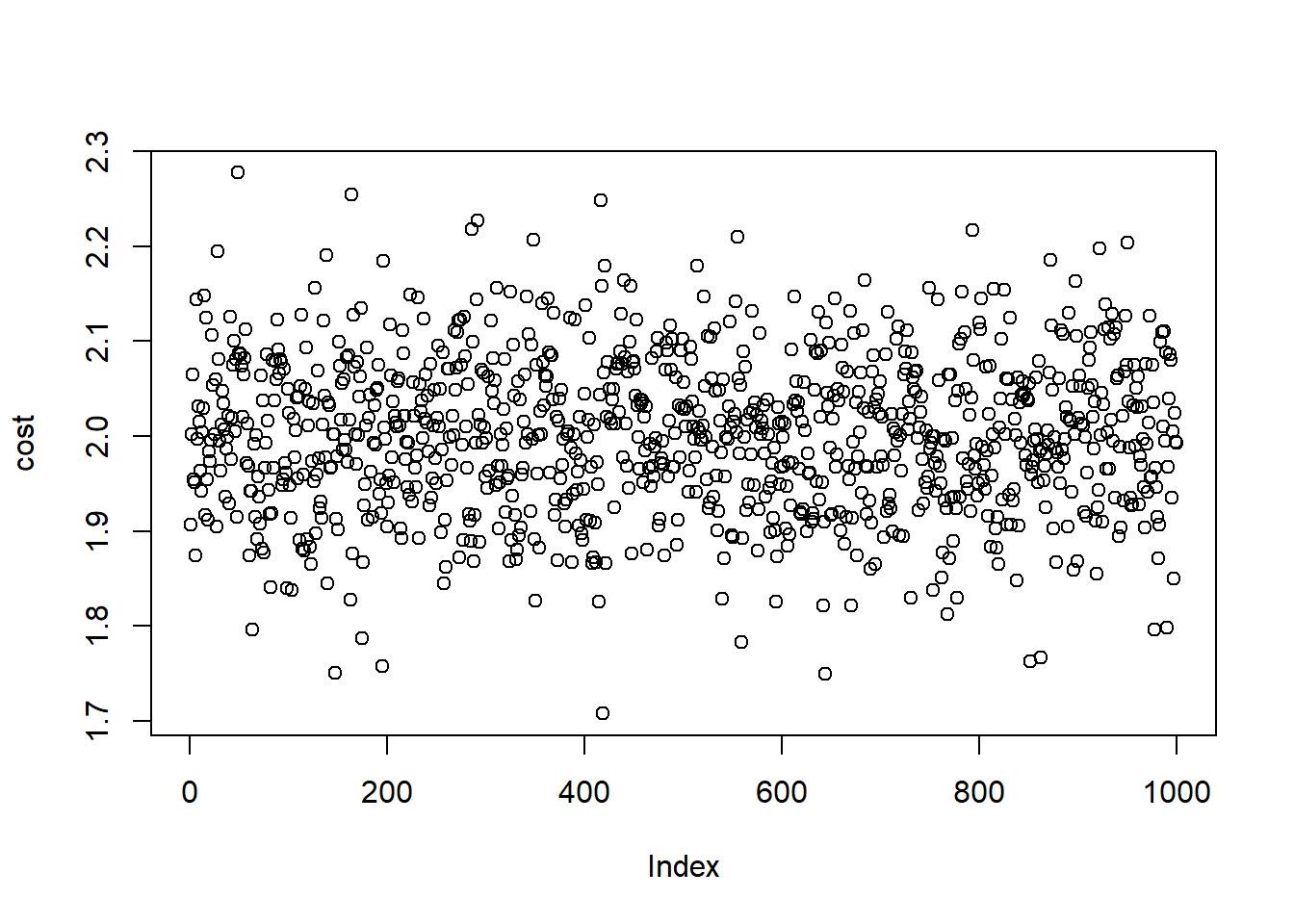

est.cost <- mean(cost)

plot(sd)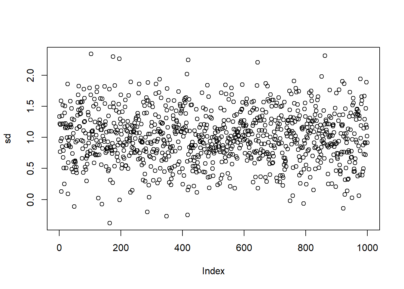

est.sd <- mean(sd)

# Final Result
cat("True cost and sd are", true.cost," and ", true.sd)

## True cost and sd are 2  and  1

cat("Estimated cost and sd are", est.cost," and ", est.sd)

## Estimated cost and sd are 2.001182  and  1.003915

Last updated on Sep 9, 2018

Edit this page