Quantmod
Quantmod stands for ``quantitative financial modelling framework’’. It has three main functions:
- download data,
- charting, and
- technical indicator.
Then we can conduct simple test on trading strategies. We will learn how to test more complicated strategies.
Before we start, let us use the following code install and load quantmod.
library(quantmod)install.packages("quantmod")
library(quantmod)Learning Objectives:
Use quantmod package to download stock prices
create chart of stock prices and add technical indicators
construct simple trading indicator and apply it into trading
evaluate the performance of a trading rule based on return data
Downloading data
Use getSymbols to get data from yahoo or Google (default is yahoo)
getSymbols("AAPL")Let see what is inside the data.
head(AAPL)## AAPL.Open AAPL.High AAPL.Low AAPL.Close AAPL.Volume AAPL.Adjusted
## 2003-01-02 0.5083427 0.5281666 0.5079888 0.5239188 45357200 0.915166
## 2003-01-03 0.5239188 0.5285210 0.5164849 0.5274589 36863400 0.921349
## 2003-01-06 0.5320605 0.5444505 0.5267507 0.5274589 97633200 0.921349
## 2003-01-07 0.5235650 0.5309990 0.5122366 0.5256886 85586200 0.918258
## 2003-01-08 0.5161310 0.5207326 0.5111750 0.5150689 57411200 0.899707
## 2003-01-09 0.5175469 0.5281666 0.5132987 0.5196706 53813200 0.907746To extract columns, we use Op, Hi, Lo, Cl, Vo and Ad
Open <- Op(AAPL)   #Open Price
High <- Hi(AAPL)    # High price
Low <- Lo(AAPL)  # Low price
Close<- Cl(AAPL)   #Close Price
Volume <- Vo(AAPL)   #Volume
AdjClose <- Ad(AAPL) # Adjusted close
If you wish to only import at a certain date e.g.,. 2000-01-01 to 2015-09-25, we can restrict the set the data to download.
getSymbols("AAPL", from='2000-01-01',to='2015-09-25')## [1] "AAPL"Alternatively, we can load the whole series and restrict using xts function last()
getSymbols("AAPL")## [1] "AAPL"AAPL <- last(AAPL,'1 year')
head(AAPL)## AAPL.Open AAPL.High AAPL.Low AAPL.Close AAPL.Volume AAPL.Adjusted
## 2020-01-02 296.24 300.60 295.19 300.35 33870100 298.8300
## 2020-01-03 297.15 300.58 296.50 297.43 36580700 295.9247
## 2020-01-06 293.79 299.96 292.75 299.80 29596800 298.2827
## 2020-01-07 299.84 300.90 297.48 298.39 27218000 296.8799
## 2020-01-08 297.16 304.44 297.16 303.19 33019800 301.6555
## 2020-01-09 307.24 310.43 306.20 309.63 42527100 308.0630Alternatively, we can take the first 3 years by using first():
getSymbols("AAPL")## [1] "AAPL"AAPL <- first(AAPL,'3 years')
head(AAPL)## AAPL.Open AAPL.High AAPL.Low AAPL.Close AAPL.Volume AAPL.Adjusted
## 2007-01-03 12.32714 12.36857 11.70000 11.97143 309579900 10.36364
## 2007-01-04 12.00714 12.27857 11.97429 12.23714 211815100 10.59366
## 2007-01-05 12.25286 12.31428 12.05714 12.15000 208685400 10.51822
## 2007-01-08 12.28000 12.36143 12.18286 12.21000 199276700 10.57016
## 2007-01-09 12.35000 13.28286 12.16429 13.22429 837324600 11.44823
## 2007-01-10 13.53571 13.97143 13.35000 13.85714 738220000 11.99609We can also import three stocks at the same time by using a vector.
getSymbols(c("AAPL","GOOG"))## [1] "AAPL" "GOOG"Alternatively, we can assign a vector of stocks and import based on the vector.
stocklist <- c("AAPL","GOOG")
getSymbols(stocklist)
The package can also import non-US stocks.
getSymbols("0941.hk")
#If error, try instead the following:
#getSymbols("0941.HK",src="yahoo", auto.assign=FALSE)head(`0941.HK`)## 0941.HK.Open 0941.HK.High 0941.HK.Low 0941.HK.Close 0941.HK.Volume
## 2007-01-02 67.25 70.00 67.10 69.6 35293388
## 2007-01-03 69.90 71.80 69.50 70.7 41163203
## 2007-01-04 70.60 70.95 67.30 68.2 37286533
## 2007-01-05 67.50 69.50 66.30 69.5 24502496
## 2007-01-08 67.50 68.40 67.45 67.7 15584163
## 2007-01-09 68.00 68.60 65.55 66.3 17861491
## 0941.HK.Adjusted
## 2007-01-02 42.11264
## 2007-01-03 42.77821
## 2007-01-04 41.26554
## 2007-01-05 42.05212
## 2007-01-08 40.96300
## 2007-01-09 40.11592Besides prices, very often we are interested in the trading volume. Moreover, we would like to find volume over time: weekly, monthly, quarterly and yearly. We can use apply and sum to calculate the rolling sum of volume to each distinct period.
WeekVoYa<- apply.weekly(Vo(AAPL),sum)
# sum from Monday to Friday
MonthVoYa <- apply.monthly(Vo(AAPL),sum)
# sum to month
QuarterVoYa <- apply.quarterly(Vo(AAPL),sum)
# sum to quarter
YearVoYa <- apply.yearly(Vo(AAPL),sum)
# sum to year
In some case, we are interested in average than the sum. Then we can use apply and mean.
WeekAveVoClYa<- apply.weekly(Vo(AAPL),mean)
# weekly average volume
Charting
Quantmod draw nice charts of following common types:
- line
- bars
- candlesticks
We can use chartSeries() and specify the types directly.
The line chart displays stock price of AAPL in 2007 by using the subset option. The option theme is set to be chartTheme(‘white’) as the default option chartTheme(‘black’) is not printer-friendly.
chartSeries(AAPL,
            type="line",
            subset='2007',
            theme=chartTheme('white'))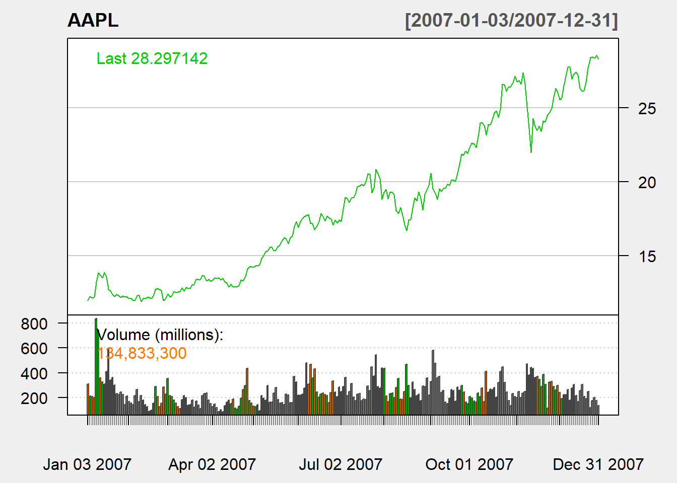
The bar chart displays stock price of AAPL in May to June 2007 by using the subset option.
chartSeries(AAPL,
            type="bar",
            subset='2007-05::2007-06',
            theme=chartTheme('white'))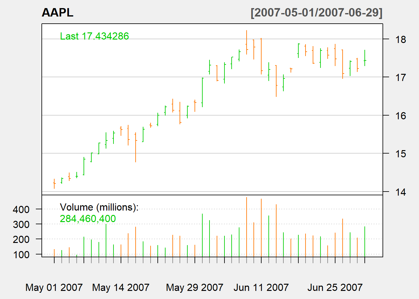
The following candle stick chart displays stock price of AAPL in May only.
chartSeries(AAPL,
            type="candlesticks",
            subset='2007-05',
            theme=chartTheme('white'))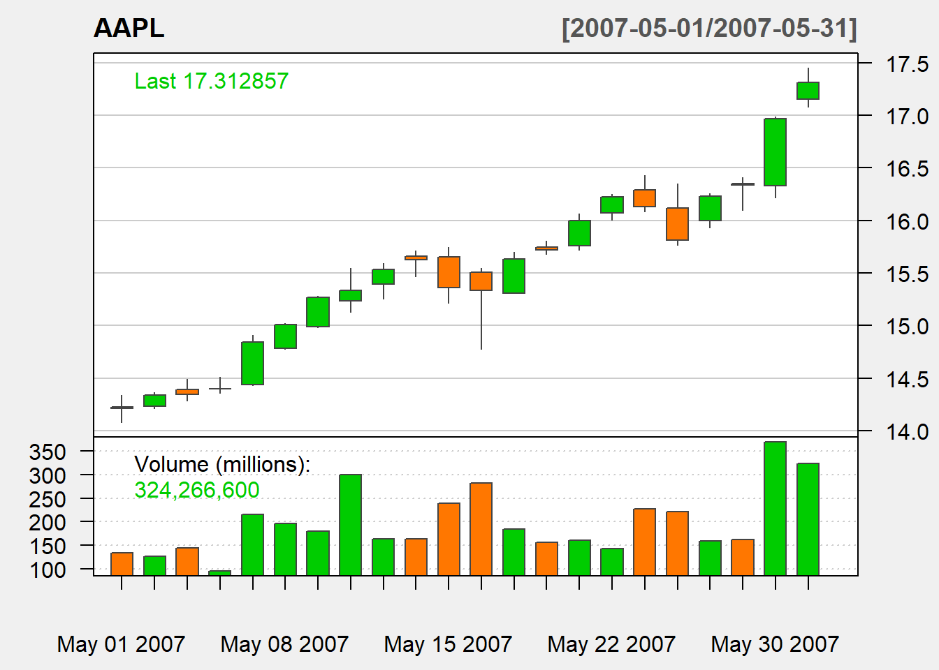
Finally The following candle stick chart displays stock price of AAPL a few days in May.
chartSeries(AAPL,
            type="auto",
            subset='2007-05-10::2007-05-30',
            theme=chartTheme('white'))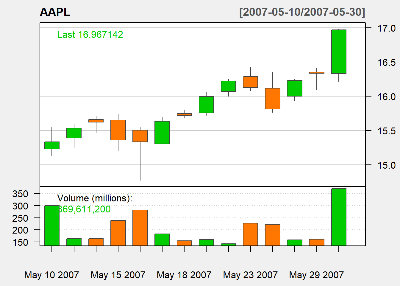
Technical Indicators
Technical trading rule (TTR) package is loaded when we load quantmod package.
If you want to use it separately, then just load the package as usual:
install.packages("TTR")
library(TTR)
Simple Moving Average
sma <-SMA(Cl(AAPL),n=20)
tail(sma,n=5)
## SMA
## 2020-06-24 339.9440
## 2020-06-25 342.2735
## 2020-06-26 344.0580
## 2020-06-29 346.0545
## 2020-06-30 348.1275Exponential moving average
ema <-EMA(Cl(AAPL),n=20)
tail(ema,n=5)
## EMA
## 2020-06-24 341.9732
## 2020-06-25 344.1510
## 2020-06-26 345.0538
## 2020-06-29 346.6468
## 2020-06-30 348.3756Bollinger band
bb <-BBands(Cl(AAPL),s.d=2)
tail(bb,n=5)
## dn mavg up pctB
## 2020-06-24 310.2851 339.9440 369.6029 0.8391221
## 2020-06-25 312.4778 342.2735 372.0692 0.8786875
## 2020-06-26 316.0863 344.0580 372.0297 0.6711018
## 2020-06-29 319.0240 346.0545 373.0850 0.7908848
## 2020-06-30 322.0402 348.1275 374.2148 0.8195523Momentum
We calculate 2-day momentum based on closing price of AAPL.
M <- momentum(Cl(AAPL), n=2)
head (M,n=5)
## AAPL.Close
## 2007-01-03 NA
## 2007-01-04 NA
## 2007-01-05 0.178571
## 2007-01-08 -0.027143
## 2007-01-09 1.074286ROC
ROC <- ROC(Cl(AAPL),n=2)
# 2-day ROC
head(ROC,n=5)
## AAPL.Close
## 2007-01-03 NA
## 2007-01-04 NA
## 2007-01-05 0.014806276
## 2007-01-08 -0.002220547
## 2007-01-09 0.084725818MACD
macd <- MACD(Cl(AAPL), nFast=12, nSlow=26,
             nSig=9, maType=SMA)
tail(macd,n=5)
## macd signal
## 2020-06-24 4.702688 3.881592
## 2020-06-25 4.600372 4.069203
## 2020-06-26 4.210396 4.195984
## 2020-06-29 4.315137 4.293894
## 2020-06-30 4.410221 4.367458RSI
rsi = RSI(Cl(AAPL), n=14)
tail(rsi,n=5)
## rsi
## 2020-06-24 68.10366
## 2020-06-25 70.22649
## 2020-06-26 60.12087
## 2020-06-29 64.15899
## 2020-06-30 65.55100Charting with Indicators
Charting SMA
We use the function addSMA() to put
chartSeries(AAPL,
            subset='2007-05::2009-01',
            theme=chartTheme('white'))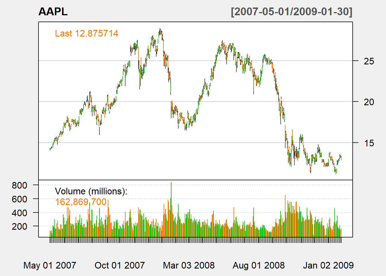
addSMA(n=30,on=1,col = "blue")
addSMA(n=200,on=1,col = "red")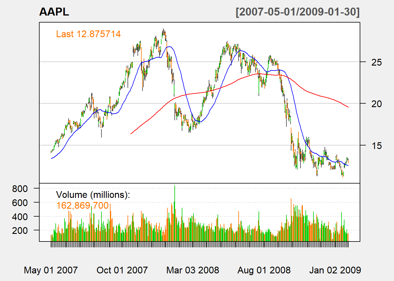
Charting EMA
chartSeries(AAPL,
            subset='2007-05::2009-01',
            theme=chartTheme('white'))
addEMA(n=30,on=1,col = "blue")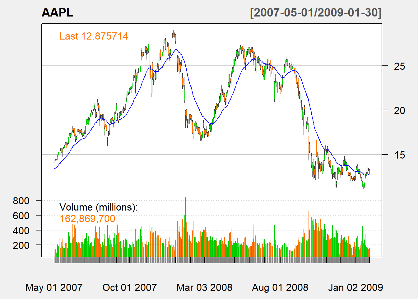
addEMA(n=200,on=1,col = "red")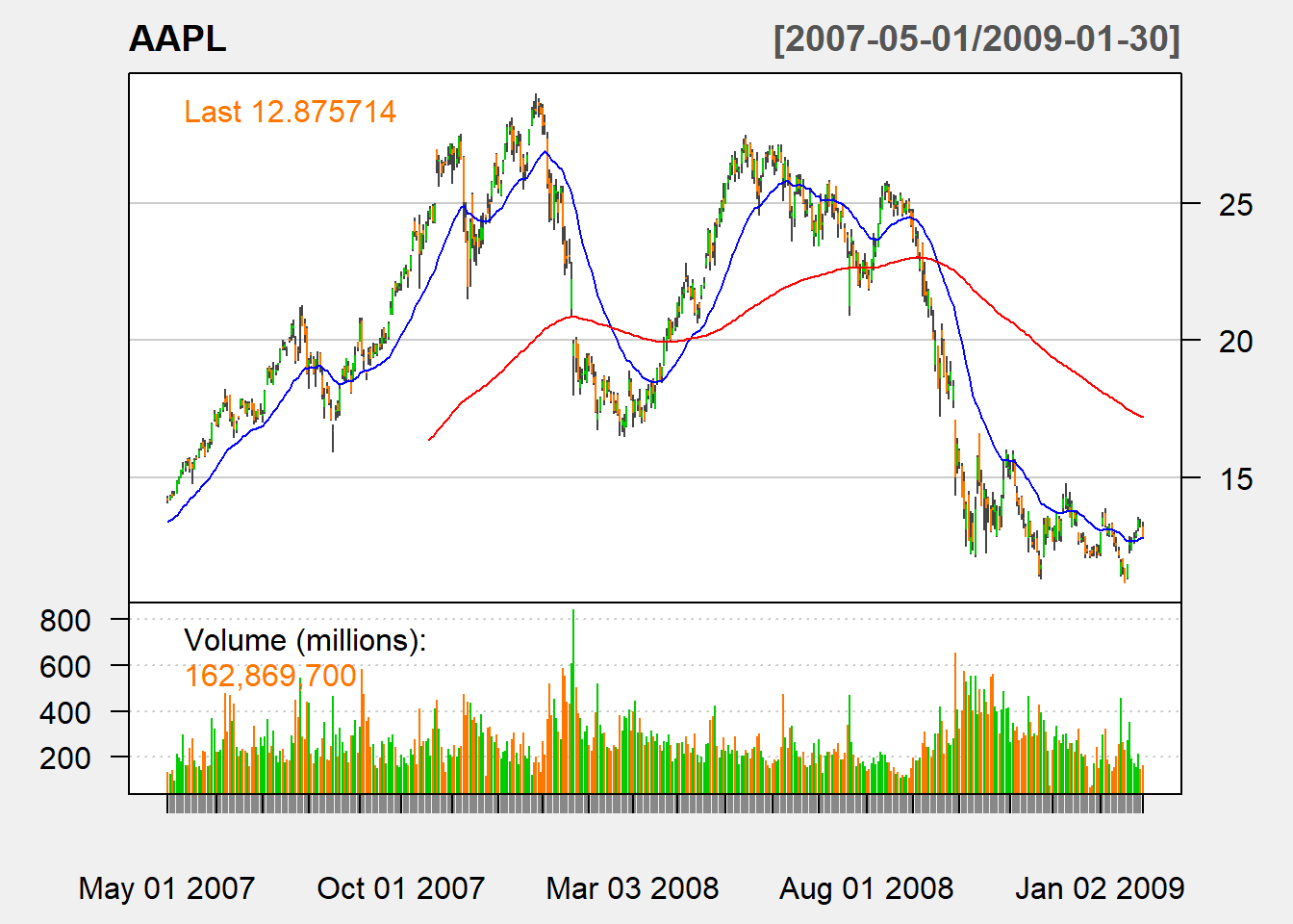
Charting Bollinger band
chartSeries(AAPL,
            subset='2007-05::2009-01',
            theme=chartTheme('white'))
addBBands(n=20,sd=2)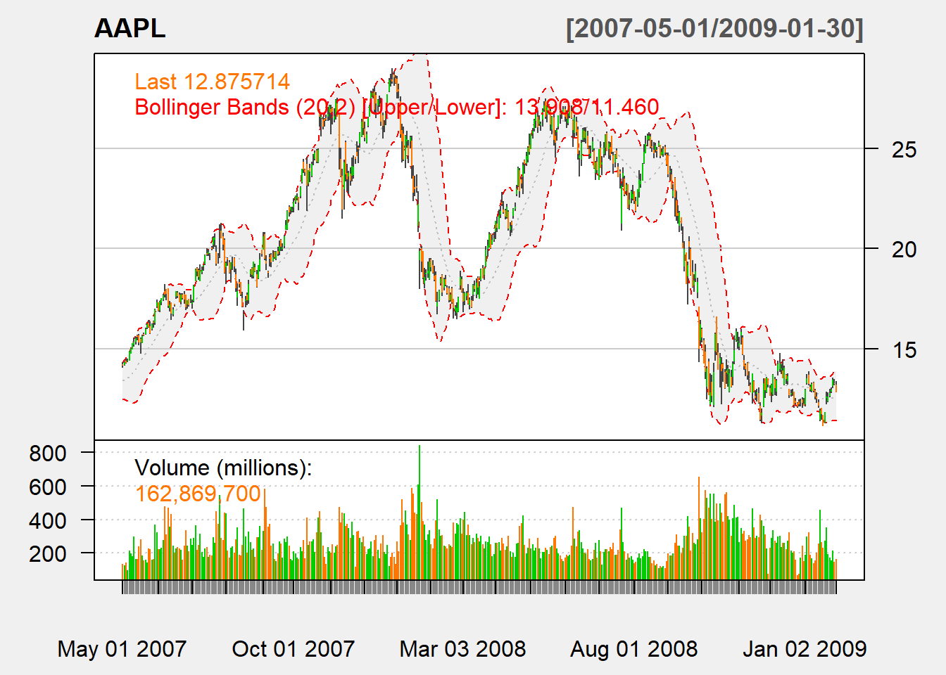
Charting Momentum
chartSeries(AAPL,
            subset='2007-05::2009-01',
            theme=chartTheme('white'))
addMomentum(n=1)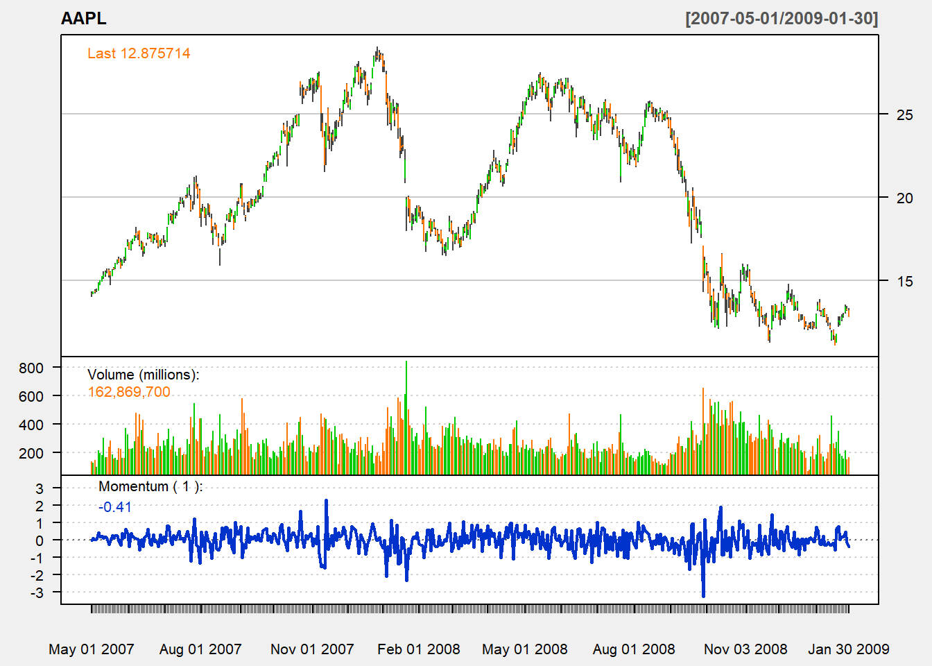
Charting ROC
chartSeries(AAPL,
            subset='2007-05::2008-01',
            theme=chartTheme('white'))
addROC(n=7)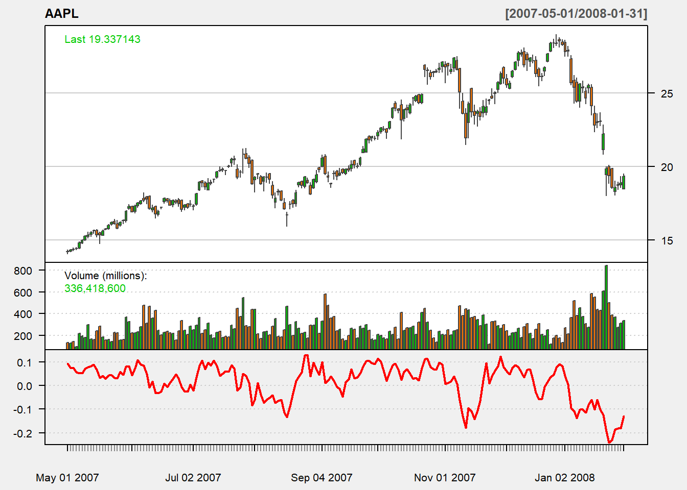
Charting MACD
chartSeries(AAPL,
            subset='2007-05::2008-01',
            theme=chartTheme('white'))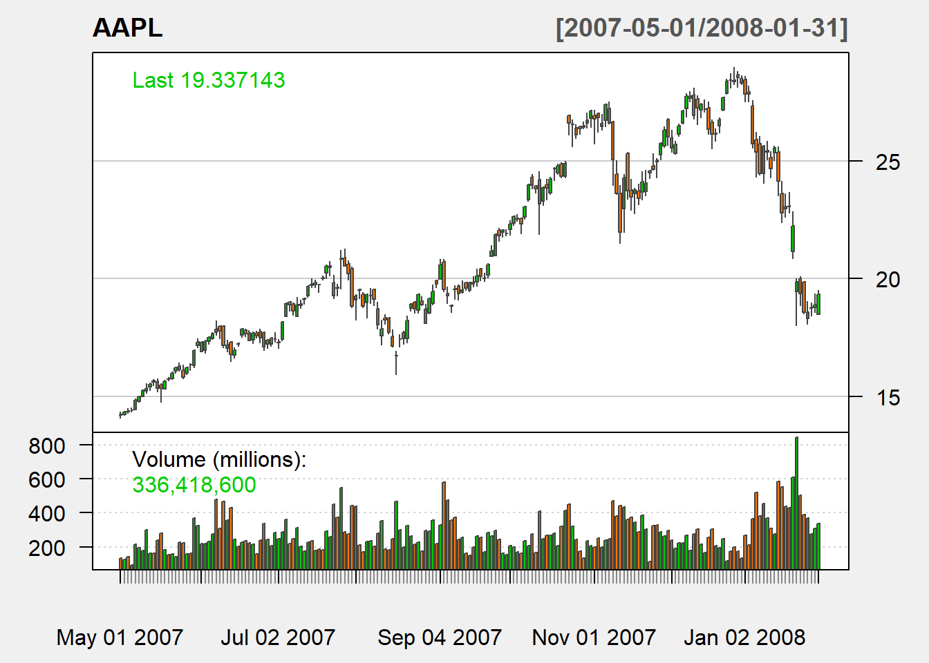
addMACD(fast=12,slow=26,signal=9,type="EMA")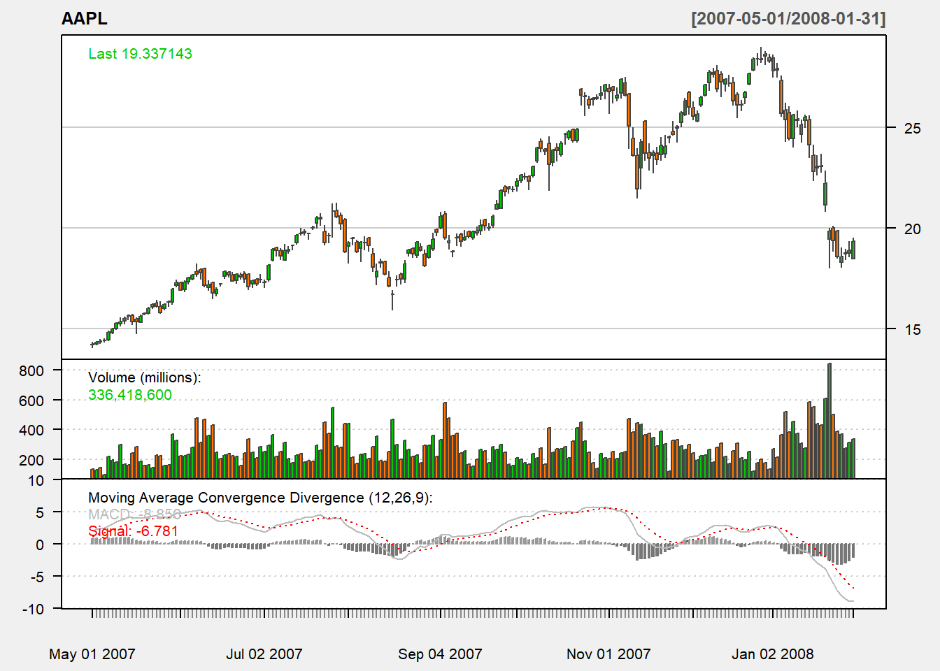
Charting RSI
chartSeries(AAPL,
            subset='2007-05::2009-01',
            theme=chartTheme('white'))
addRSI(n=14,maType="EMA")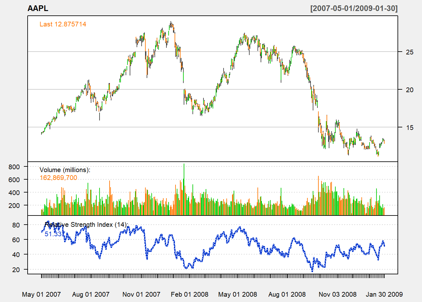
Charting Custom TA
sma <- SMA(Cl(AAPL),n=14)
chartSeries(AAPL,
            subset='2007-05::2009-01',
            theme=chartTheme('white'))
addTA(sma, on=1, col="red")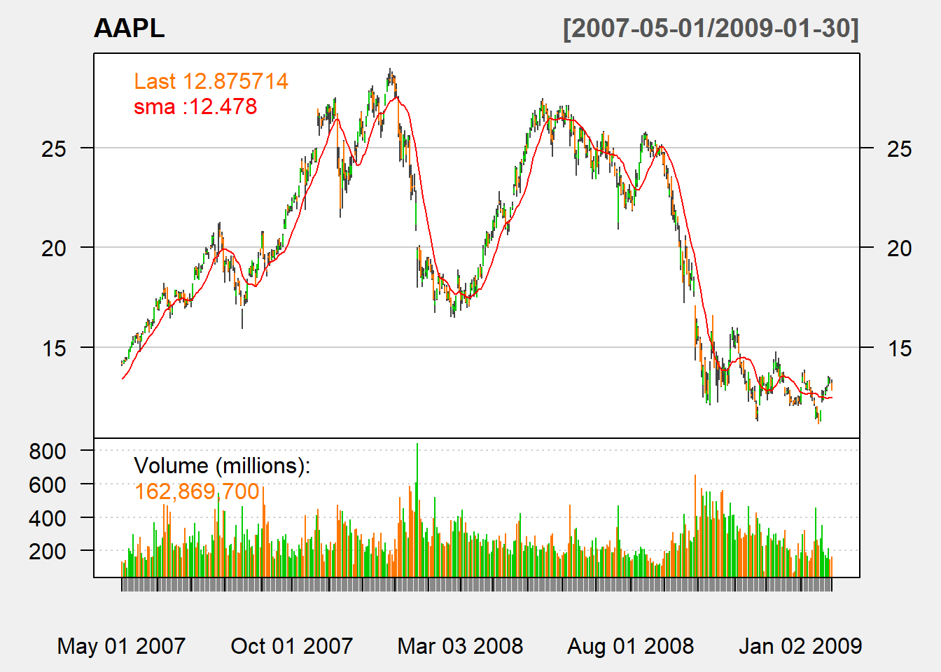
Charting Price changes of two stocks
To compare prices fo different stocks, we need to calculat the price change:
NS <- function(xdat) xdat / coredata(xdat)[1]
a <- NS(Cl(AAPL))-1
g <- NS(Cl(GOOG))-1
m <- NS(Cl(MSFT))-1
chartSeries(a,
            subset = '2007',
            theme=chartTheme('white'))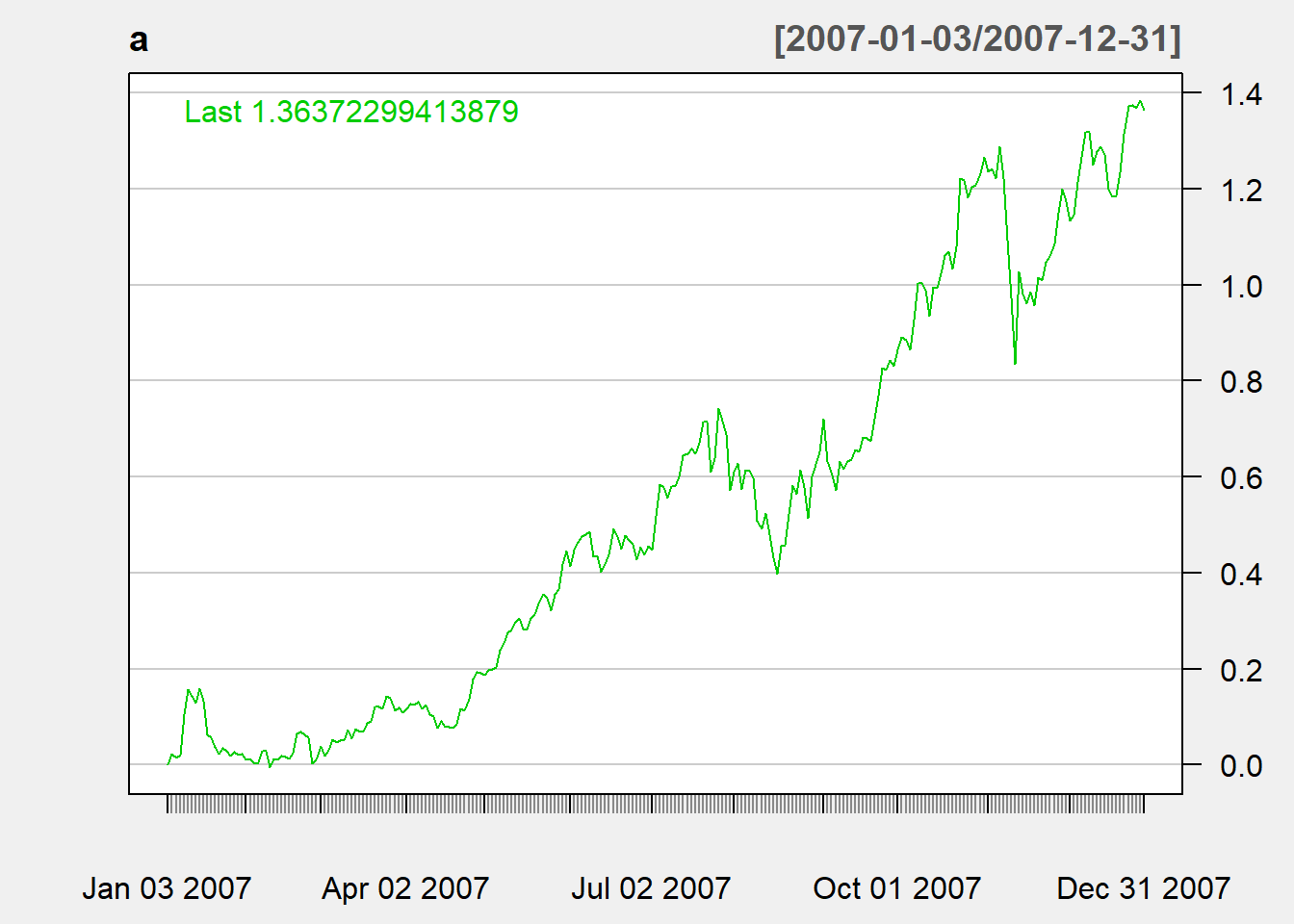
addTA(g, on=1, col="red", lty="dotted")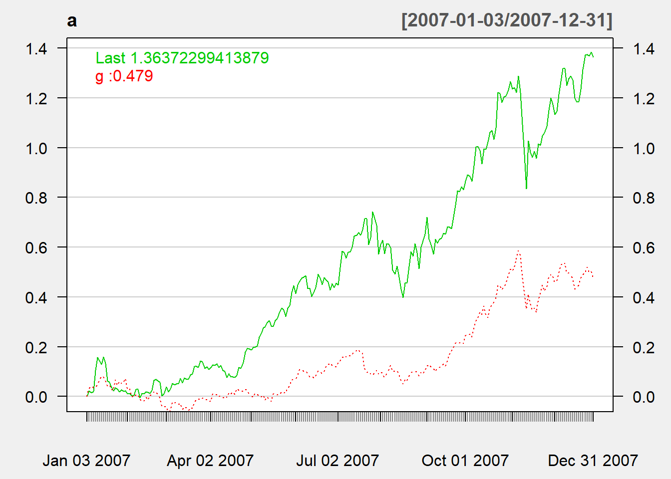
addTA(m, on=1, col="blue", lty="dashed")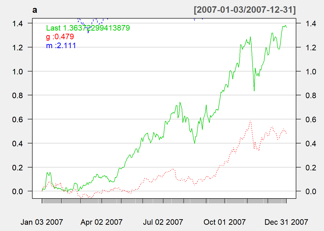
The option lty is to make the line becomes other line styles where dotted means dotted line and dashed means dashed line.
Performance Evaluation
The package is a collection of econometric functions for performance and risk analysis.
We first install and load PerformanceAnalytics package.
install.packages("PerformanceAnalytics")
library(PerformanceAnalytics)
Evaluating Trading Rules
To simplify, we first evaluate several trading rules based on day trading:
- buy signal based on simple filter rule
- buy and sell signals based on simple filter rule
- buy signal based on RSI
- buy signal based on EMA and sell signal based on RSI
- buy signal based on RSI but trading size depends on price history
Finally, we consider the rule that does non-day trading. In this case, we need to keep track of both cash and stock holdings.
Simple filter Buy
Here we create trading signal based on simple filter rule. Recall that simple filter rule suggests buying when the price increases a lot compared to the yesterday price: \[\begin{align*} \text{Buy}&:\frac{P_t}{P_{t-1}}>1+\delta \\ \end{align*}\] where \(P_t\) is the closing price at time \(t\) and \(\delta>0\) is an arbitrary threshold
We illustrate using Microsoft with ticker MSFT.
We first download the data using getSymbols(“MSFT”).
library(quantmod)
getSymbols("MSFT")
## [1] "MSFT"We first will use closing price to perform calculation. We calculate the percentage price change by dividing the current close price by its own lag and then minus 1.
Now we generate buying signal based on filter rule:
price <- Cl(MSFT) # close price
r <- price/Lag(price) - 1 # % price change
delta <-0.005 #threshold
signal <-c(0) # first date has no signal

#Loop over all trading days (except the first)
for (i in 2: length(price)){
  if (r[i] > delta){
    signal[i]<- 1
  } else
    signal[i]<- 0
}
Note that signal is just a vector without time stamp. We use the function reclass to convert it into an xts object.
# Each data is not attached with time
head(signal, n=3)
## [1] 0 0 0# Assign time to action variable using reclass;
signal<-reclass(signal,price)
# Each point is now attached with time
tail(signal, n=3)## [,1]
## 2020-06-26 0
## 2020-06-29 1
## 2020-06-30 1We are now ready to chart the trading indicators:
# Charting with Trading rule
chartSeries(MSFT,
            type = 'line',
            subset="2009-08::2009-09-15",
            theme=chartTheme('white'))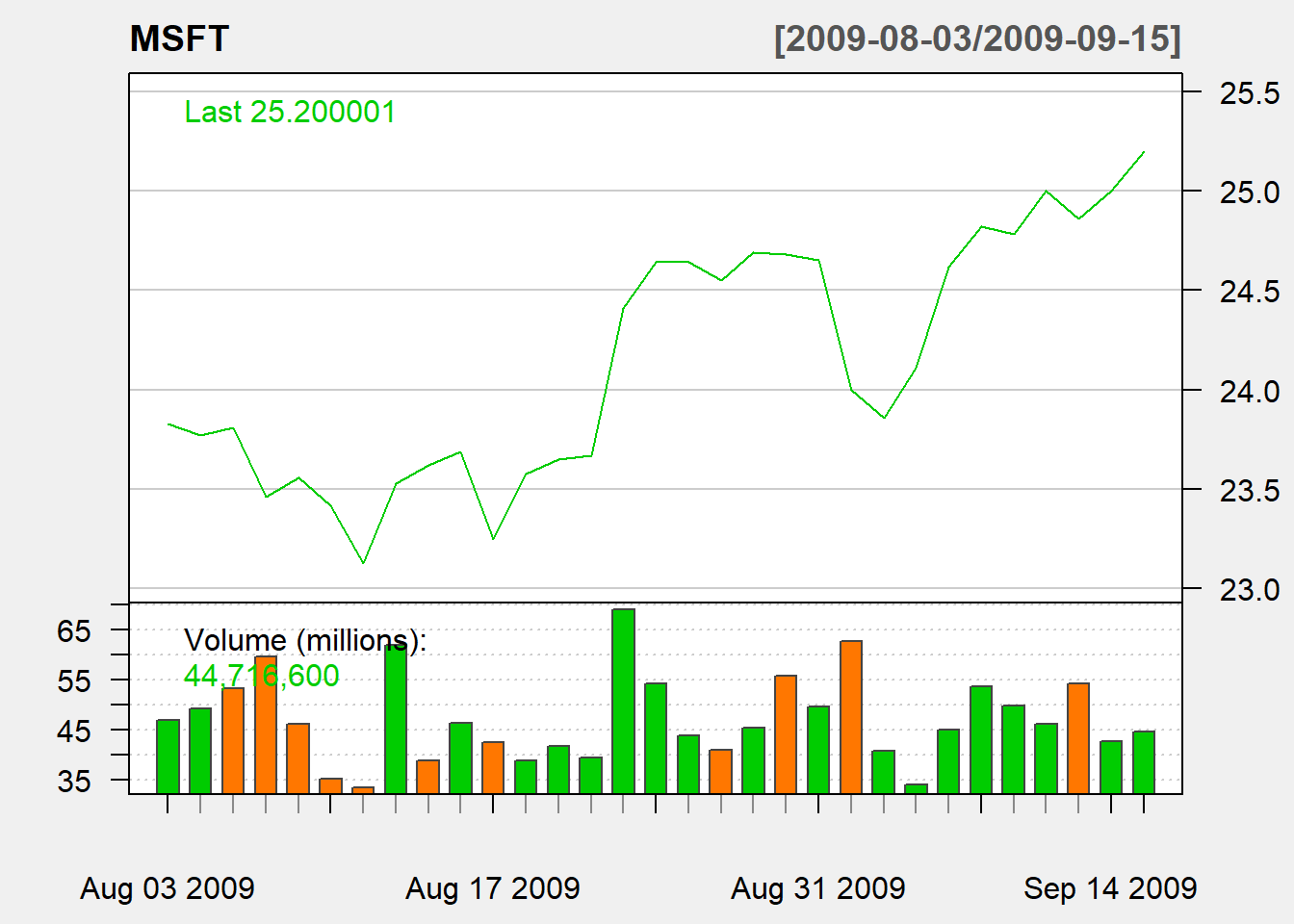
addTA(signal,type='S',col='red')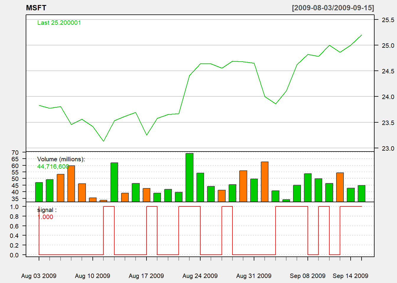
We consider trading based on yesterday indicator:
trade <- Lag(signal,1) # trade based on yesterday signalTo keep it simple, we evaluate using day trading:
- buy at open
- sell at close
- trading size: all in
Then daily profit rate is \(dailyReturn=\frac{Close - Open}{open}\)
ret<-dailyReturn(MSFT)*trade
names(ret)<-"filter"
Based on daily return, we can see the summary of performance using charts.PerformanceSummary() to evaluate the performance.
#Performance Summary
charts.PerformanceSummary(ret, main="Naive Buy Rule")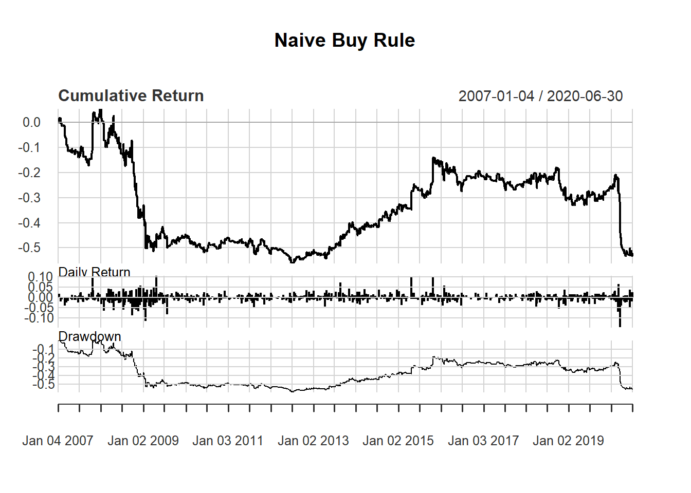
Simple fiter buy-sell
Here we create trading signal based on simple filter rule. Recall that simple filter rule suggests buying when the price increases a lot compared to the yesterday price and selling when price decreases a lot: \[\begin{align*} \text{Buy}&:\frac{P_t}{P_{t-1}}>1+\delta \\ \text{Sell}&:\frac{P_t}{P_{t-1}}<1-\delta \end{align*}\] where \(P_t\) is the closing price at time \(t\) and \(\delta>0\) is an arbitrary threshold
We first download the data:
library(quantmod)
getSymbols("MSFT")
## [1] "MSFT"price <- Cl(MSFT)
r <- price/Lag(price) - 1
delta<-0.005
signal <-c(NA) # first signal is NA
for (i in 2: length(Cl(MSFT))){
if (r[i] > delta){
signal[i]<- 1
} else if (r[i]< -delta){
signal[i]<- -1
} else
signal[i]<- 0
}
signal<-reclass(signal,Cl(MSFT))
trade1 <- Lag(signal)
ret1<-dailyReturn(MSFT)*trade1
names(ret1) <- 'Naive'
charts.PerformanceSummary(ret1)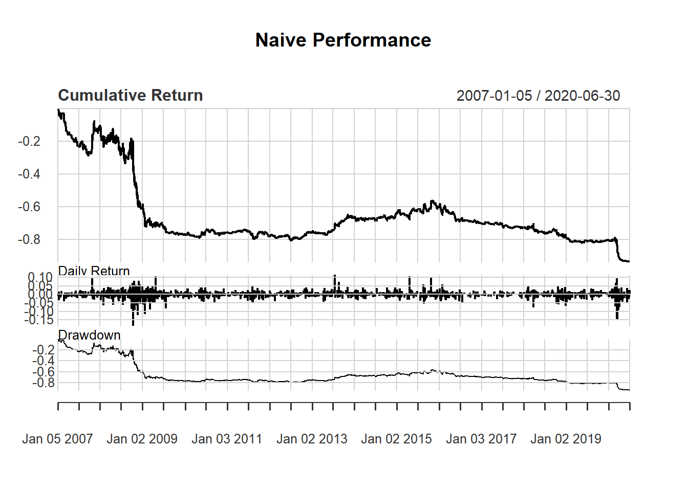
Exercise
Test the following strategy based on EMA: - Buy/Sell signal based on EMA rule. - Day trading based on yesterday signal: - buy at open and - sell at close on the same day
An example using RSI
Consider following day-trading strategy based on 14-day RSI:
- buy one unit if RSI <30 and
- otherwise no trade.
Evaluate this based on day trading and compare it with simple filter rule:
day <-14
price <- Cl(MSFT)
signal <- c()                    #initialize vector
rsi <- RSI(price, day)     #rsi is the lag of RSI
signal [1:day+1] <- 0            #0 because no signal until day+1

for (i in (day+1): length(price)){
  if (rsi[i] < 30){             #buy if rsi < 30
    signal[i] <- 1
  }else {                       #no trade all if rsi > 30
    signal[i] <- 0
  }
}
signal<-reclass(signal,Cl(MSFT))
trade2 <- Lag(signal)

#construct a new variable ret1
ret1 <- dailyReturn(MSFT)*trade1
names(ret1) <- 'Naive'
# construct a new variable ret2
ret2 <- dailyReturn(MSFT)*trade2
names(ret2) <- 'RSI'
Now compare strategies with the filter rule:
retall <- cbind(ret1, ret2)
charts.PerformanceSummary(retall,
                          main="Naive v.s. RSI")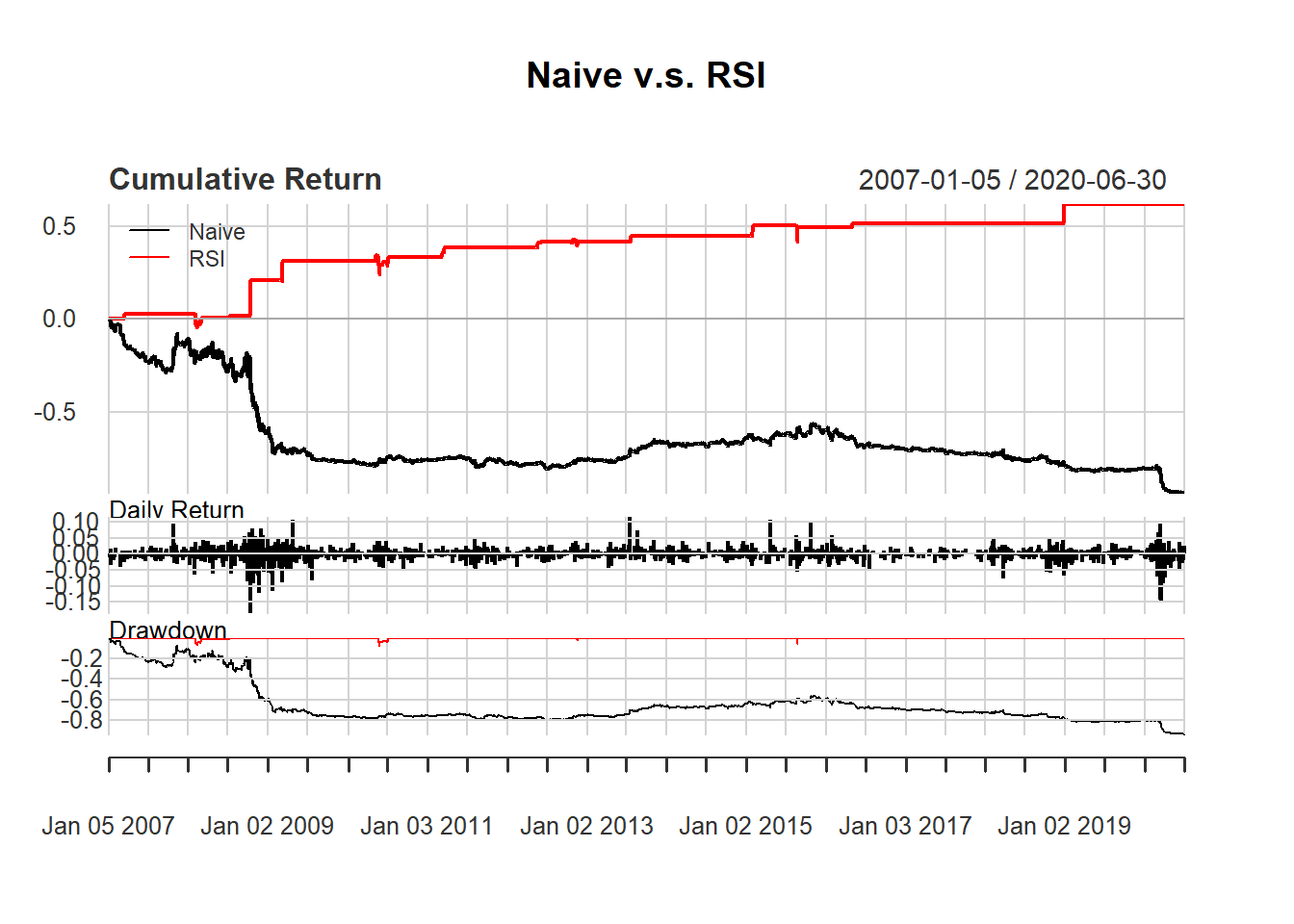
More efficient code
In the RSI code above, we have written that:
signal [1:day+1] <- 0

for (i in (day+1): length(price)){
  if (rsi[i] < 30){
    signal[i] <- 1
  }else {
    signal[i] <- 0
  }
}
A more efficient but less readable code is to avoid counting:
for (i in 1:length(price)){
  signal[i] <- 0
  if (isTRUE(rsi[i] < 30)){
    signal[i] <- 1
  }
}
Combining two indicators: filter and RSI
Test the following strategy using filter and RSI based on day trading:
Buy signal based on filter rule.
Sell signal based on RSI rule.
Tie-breaking: buy-signal has priority
We use 14-day RSI and use 70 as threshold for selling.
n <- 14
delta<-0.005
price <- Cl(MSFT)
r <- price/Lag(price) - 1
rsi <- RSI(price, n)
signal <-c()    # first signal is NA
signal[1:n] <-0


# Generate Trading Signal
for (i in (n+1):length(price)){
    if (r[i] > delta){
         signal[i]<- 1
    } else if (rsi[i] > 70){
         signal[i]<- -1
    } else
         signal[i]<- 0
}
signal<-reclass(signal,price)

## Apply Trading Rule
trade3 <- Lag(signal)
ret3<-dailyReturn(MSFT)*trade3
names(ret3) <- 'Combine'
retall <- cbind(ret1, ret2, ret3)
To draw trade performance summary with different colors, we use the option colorset. Common options includes redfocus, bluefocus, greenfocus, rainbow4equal andrich12equal.
charts.PerformanceSummary(
  retall, main="Naive v.s. RSI v.s. Combine",
  colorset=bluefocus)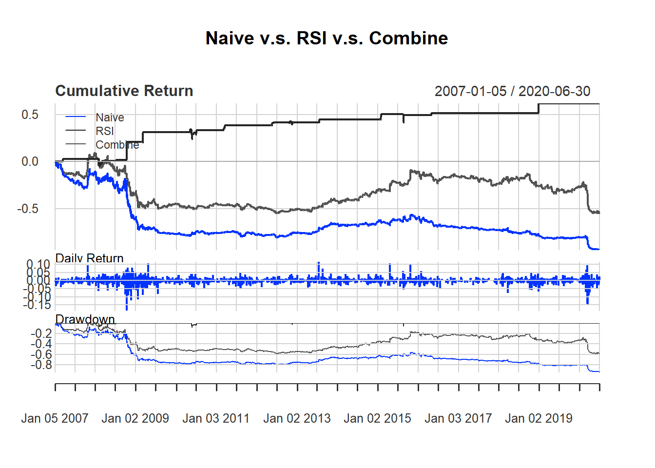
Exercise
Test the following strategy based on EMA and RSI
Buy signal based on EMA rule.
Sell signal based on RSI rule
Day trading based on yesterday signal: buy at open and sell at close
Trading Size
Wealth: 1 million
Trade unit: 1000 stocks per trade
Test the following strategy based on 14-day RSI :
Buy one more unit if RSI <30.
Keep buying the same if 30 < RSI < 50
Stop trading if RSI >= 50
Evaluate based on day trading
To take trade size into account, we need to keep track of wealth:
qty <-1000
day <-14

signal <- c()    #trade signal with size
signal[1:(day+1)] <- 0

price <- Cl(MSFT)

wealth <-c()
wealth[1:(day+1)] <- 1000000

return<-c()
return[1:(day+1)] <- 0

profit <-c()
profit[1:(day+1)] <- 0
We now generate trading signal with size:
rsi <- RSI(price, day)  #rsi is the lag of RSI
for (i in (day+1): length(price)){
  if (rsi[i] < 30){  #buy one more unit if rsi < 30
    signal[i] <- signal[i-1]+1
  } else if (rsi[i] < 50){  #no change if rsi < 50
    signal[i] <- signal[i-1]
  } else {         #sell  if rsi > 50
    signal[i] <- 0
  }
}
signal<-reclass(signal,price)
Now we are ready to apply Trade Rule
Close <- Cl(MSFT)
Open <- Op(MSFT)
trade <- Lag(signal)
for (i in (day+1):length(price)){
  profit[i] <- qty * trade[i] * (Close[i] - Open[i])
  wealth[i] <- wealth[i-1] + profit[i]
  return[i] <- (wealth[i] / wealth[i-1]) -1
}
ret3<-reclass(return,price)

charts.PerformanceSummary(ret3, main="Trade Size")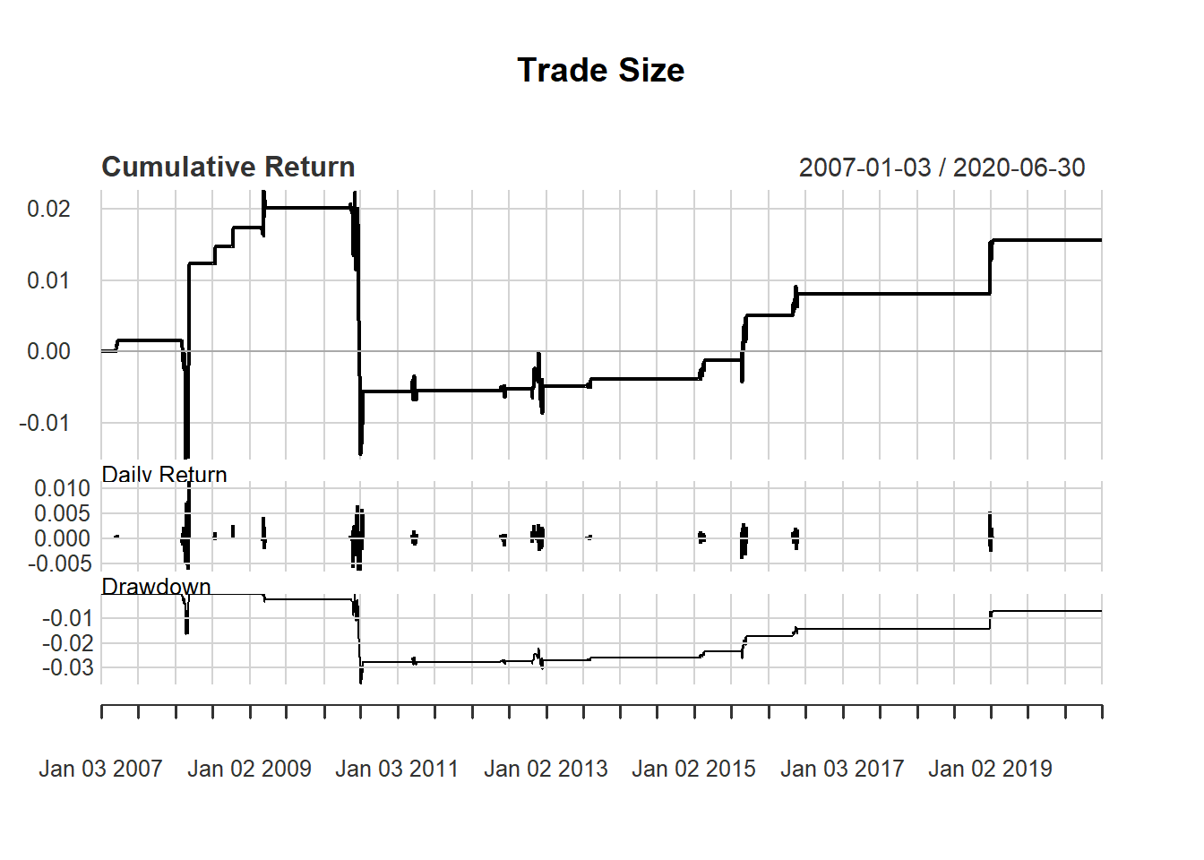
Non-Day Trading
Trading signal:
Buy signal arises if 14-day RSI < 30
Sell signal arises if 14-day RSI > 50
Trading Rule
Buy 300 units under buy signal
Sell all when sell signal appears
Initial wealth: 10,000
Note that we need to keep track of both cash and stock holdings.
qty <-300
day <-14

signal <- c()   #trade signal
signal[1:(day+1)] <- 0

price <- Cl(MSFT)

stock <- c()  #stock holding
stock[1:(day+1)] <-0

cash <-c()
cash[1:(day+1)] <- 10000
Trading signal is based on simple RSI:
rsi <- RSI(price, day)  #rsi is the lag of RSI
for (i in (day+1): length(price)){
  if (rsi[i] < 30){  #buy one more unit if rsi < 30
    signal[i] <- 1
  } else if (rsi[i] < 50){ #no change if rsi < 50
    signal[i] <- 0
  } else {         #sell  if rsi > 50
    signal[i] <- -1
  }
}
signal<-reclass(signal,price)
Assume buying at closing price. We keep track of how cash and stock changes:
trade <- Lag(signal)    #rsi is the lag of RSI
for (i in (day+1): length(price)){
  if (trade[i]>=0){
    stock[i] <- stock[i-1] + qty*trade[i]
    cash[i] <- cash[i-1] -
      qty*trade[i]*price[i]
  } else{
    stock[i] <- 0
    cash[i] <- cash[i-1] +
      stock[i-1]*price[i]
  }
}
stock<-reclass(stock,price)
cash<-reclass(cash,price)
To evaluate performance, we calculate equity using cash and stock holdings.
equity <-c()
equity[1:(day+1)] <- 10000

return<-c()
return[1:(day+1)] <- 0

for (i in (day+1): length(price)){
  equity[i] <- stock[i] * price[i] + cash[i]
  return[i] <- equity[i]/equity[i-1]-1
}
equity<-reclass(equity,price)
return<-reclass(return,price)
Performance Charts
charts.PerformanceSummary(return,
                          main="Non-Day-Trading")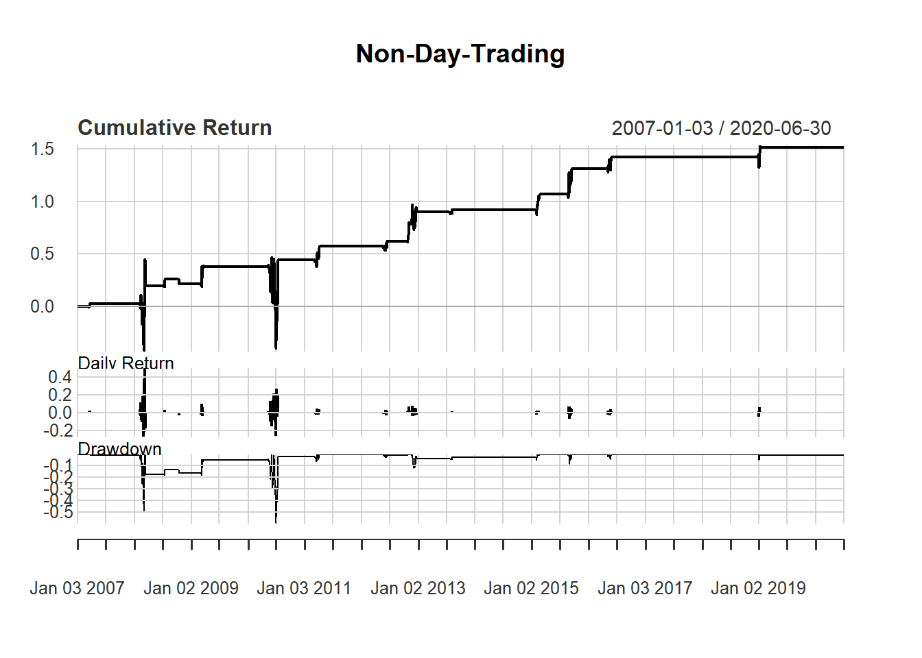
We can plot the equity line showing how the performance of the strategy:
chart_Series(equity, main="equity line")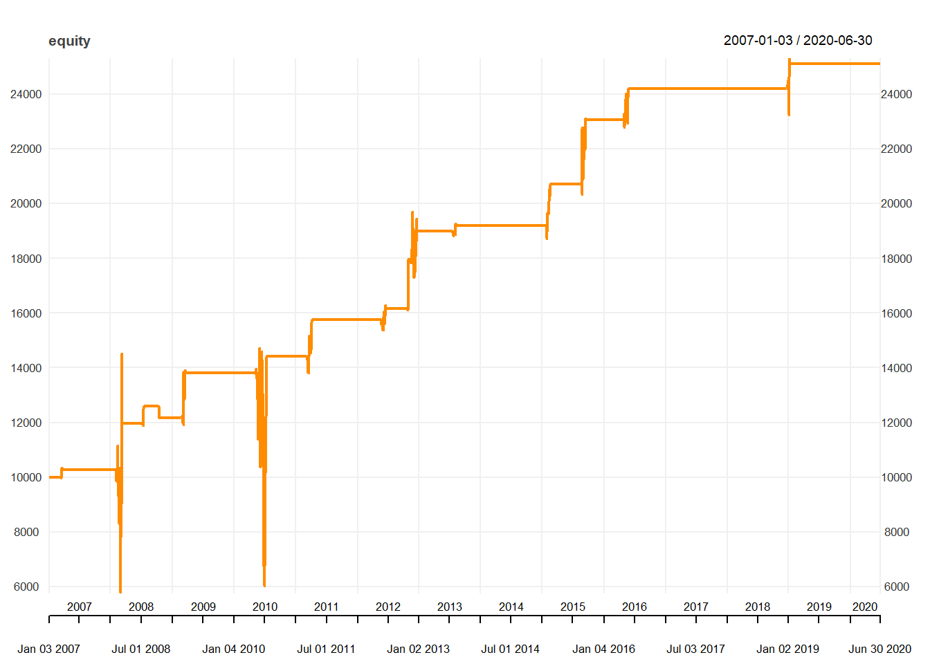
We can check the cash account over time:
chart_Series(cash, name="Cash Holding")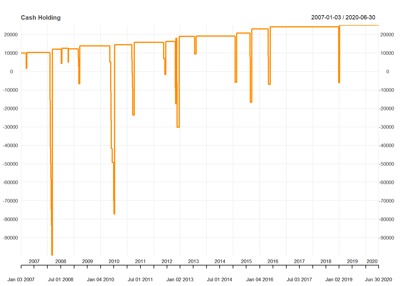
Finall, We can stock holdings:
chart_Series(stock, name="Stock Holding")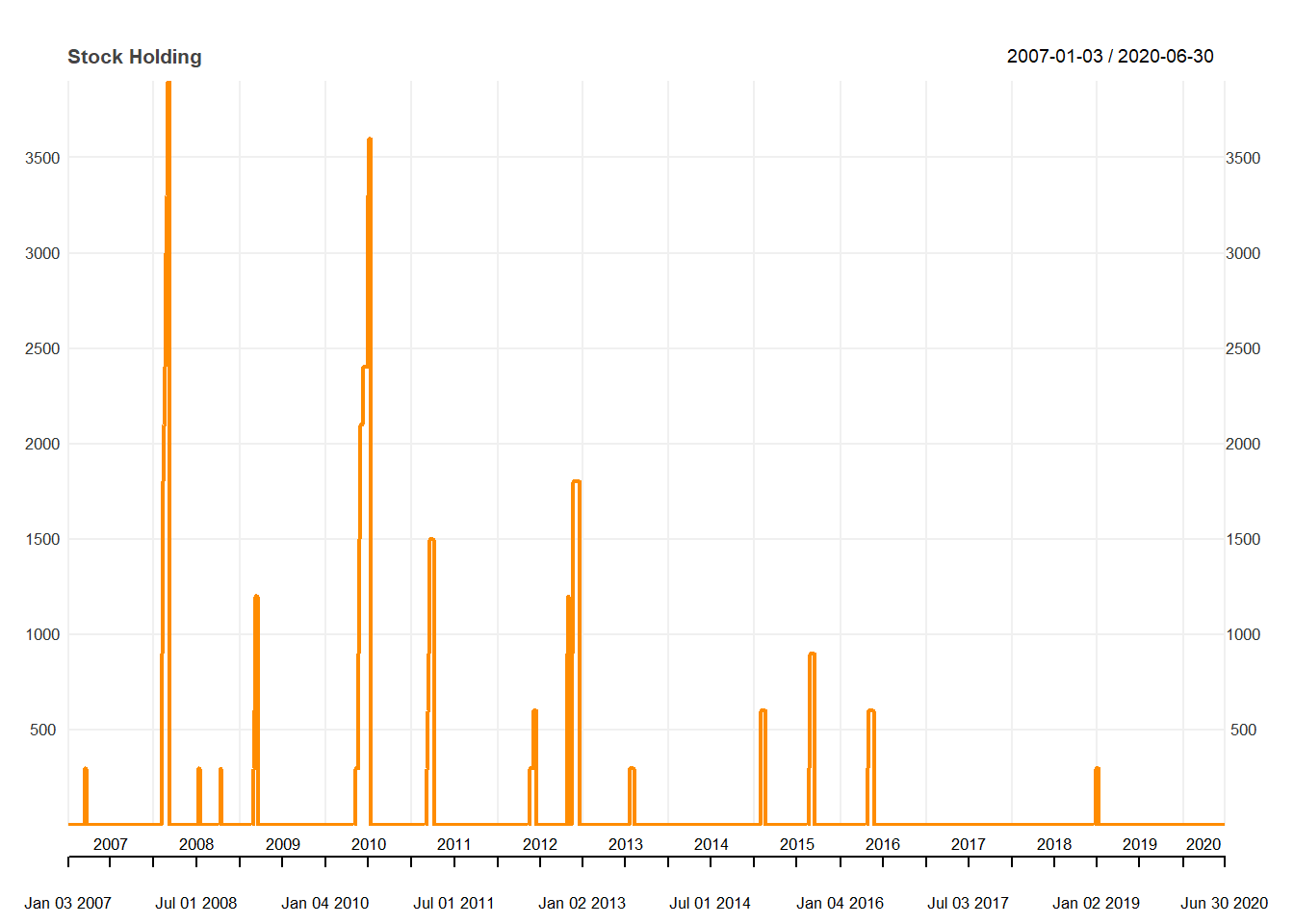
Exercise
Trading signal:
Buy signal arises if RSI < 30
Sell signal arises if RSI >50
Trading Rule
Buy 1000 units under buy signal
Sell 1000 units under sell signal