Quanstrat
Since quantstrat is not standard package, we first learn how to install custom package.
We will illustrate the usage of the quantstrat package by showing how four different rules be applied:
- naive filter rule,
- buy and hold,
- simple SMA rule,
- SMA rule with a volatility filter.
Since the coding is complicated, we first overview the structure of the code. There are five parts:
- Initialization
- Indicator: filter rule/SMA rule
- Signals: buy/sell signals
- Rule: buy or sell? quantity?
- Evaluation of results.
Before we start, let us make sure that we have installed the following four standard packages:
- quantmod,
- PerformanceAnalytics,
- FinancialInstrument, and
- foreach.
If your R does not have them, please run the following code:
install.packages("quantmod")
install.packages("FinancialInstrument")
install.packages("PerformanceAnalytics")
install.packages("foreach")
FinancialInstrument allows you to specify your assets class (e.g., stock, derivatives, currency) and foreach is a package that allow fast computation (i.e., parallel computation).
Install custom packages
Since blotter and quanstrat are still under development, they are not yet available at CRAN. We need to install the two package from github. We need to install devtools package first.
Then we use the function install_github to download the packages, and then we load them into the system.
install.packages("devtools")
library(devtools)
# Install from github directly
install_github("braverock/blotter")
install_github("braverock/quanstrat")
library(blotter)
library(quantstrat)
IF there is an error during installation process, try again after installing the latest R and update all packages.
Blotter Package
Since working through quanstrat package requires the blotter package, which is rather complicated, we demostrate first how the blotter pacakge works first.
As we have seen, recording tranasction of stocks, keeping track of cash and stock holding, and evaluate return is rather messy. The blotter package is mainly for this purpose.
We first need to setup the working space.
We need to setup the currency and declare the data is the stock (using FinancialInstrument package).
The multipler is always one for stock, and currency is USD for US stock.
options("getSymbols.warning4.0"=FALSE)
from ="2008-01-01"
to ="2012-12-31"
symbols = c("AAPL", "IBM")
currency("USD")
getSymbols(symbols, from=from, to=to,
           adjust=TRUE)
stock(symbols, currency="USD", multiplier=1)
initEq=10^6
To start, we initialize account and portfolio where:
Porfolio: stores which stocks to be traded
Account: stores which money transactions
rm("account.buyHold",pos=.blotter)
rm("portfolio.buyHold",pos=.blotter)

initPortf("buyHold", symbol=symbols)
initAcct("buyHold", portfolios = "buyHold",
         initEq = initEq)
Buy and hold
To illustrate, we just consider buy and hold strategy:
- Buy on the first day at closing price
- Sell on the last day at closing price
We first get the price and timing data:
Apple.Buy.Date <- first(time(AAPL))
Apple.Buy.Price <- as.numeric(Cl(AAPL[Apple.Buy.Date,]))
Apple.Sell.Date <- last(time(AAPL))
Apple.Sell.Price <- as.numeric(Cl(AAPL[Apple.Sell.Date,]))
Apple.Qty <- trunc(initEq/(2*Apple.Buy.Price))

IBM.Buy.Date <- first(time(IBM))
IBM.Buy.Price <- as.numeric(Cl(IBM[IBM.Buy.Date,]))
IBM.Sell.Date <- last(time(IBM))
IBM.Sell.Price <- as.numeric(Cl(IBM[IBM.Sell.Date,]))
IBM.Qty <- trunc(initEq/(2*IBM.Buy.Price))
We first add buy transactions to the system using the function addTxn:
addTxn(Portfolio = "buyHold",
       Symbol = "AAPL",
       TxnDate = Apple.Buy.Date,
       TxnQty = Apple.Qty,
       TxnPrice = Apple.Buy.Price,
       TxnFees = 0)

addTxn(Portfolio = "buyHold",
       Symbol = "IBM",
       TxnDate = IBM.Buy.Date,
       TxnQty = IBM.Qty,
       TxnPrice = IBM.Buy.Price,
       TxnFees = 0)
Then we add the sell transactions:
addTxn(Portfolio = "buyHold",
       Symbol = "AAPL",
       TxnDate = Apple.Sell.Date,
       TxnQty = -Apple.Qty,
       TxnPrice = Apple.Sell.Price,
       TxnFees = 0)

addTxn(Portfolio = "buyHold",
       Symbol = "IBM",
       TxnDate = IBM.Sell.Date,
       TxnQty = -IBM.Qty,
       TxnPrice = IBM.Sell.Price,
       TxnFees = 0)
Now we can update the account based on the added transactions:
updatePortf(Portfolio = "buyHold")## [1] "buyHold"updateAcct(name = "buyHold")## [1] "buyHold"updateEndEq(Account = "buyHold")## [1] "buyHold"We can chart our trading positions:
chart.Posn("buyHold", Symbol = "AAPL")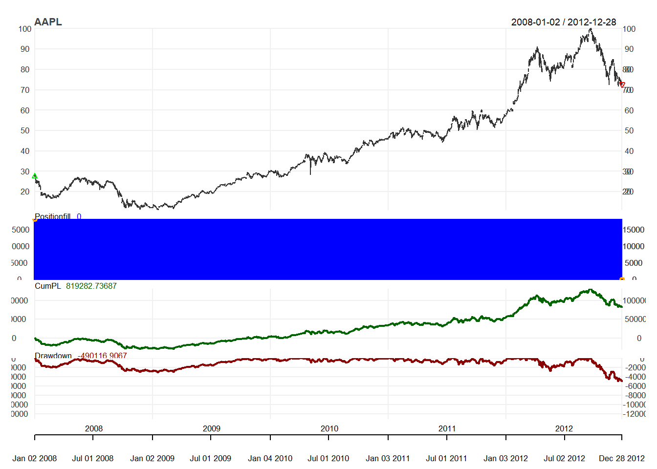
chart.Posn("buyHold", Symbol = "IBM")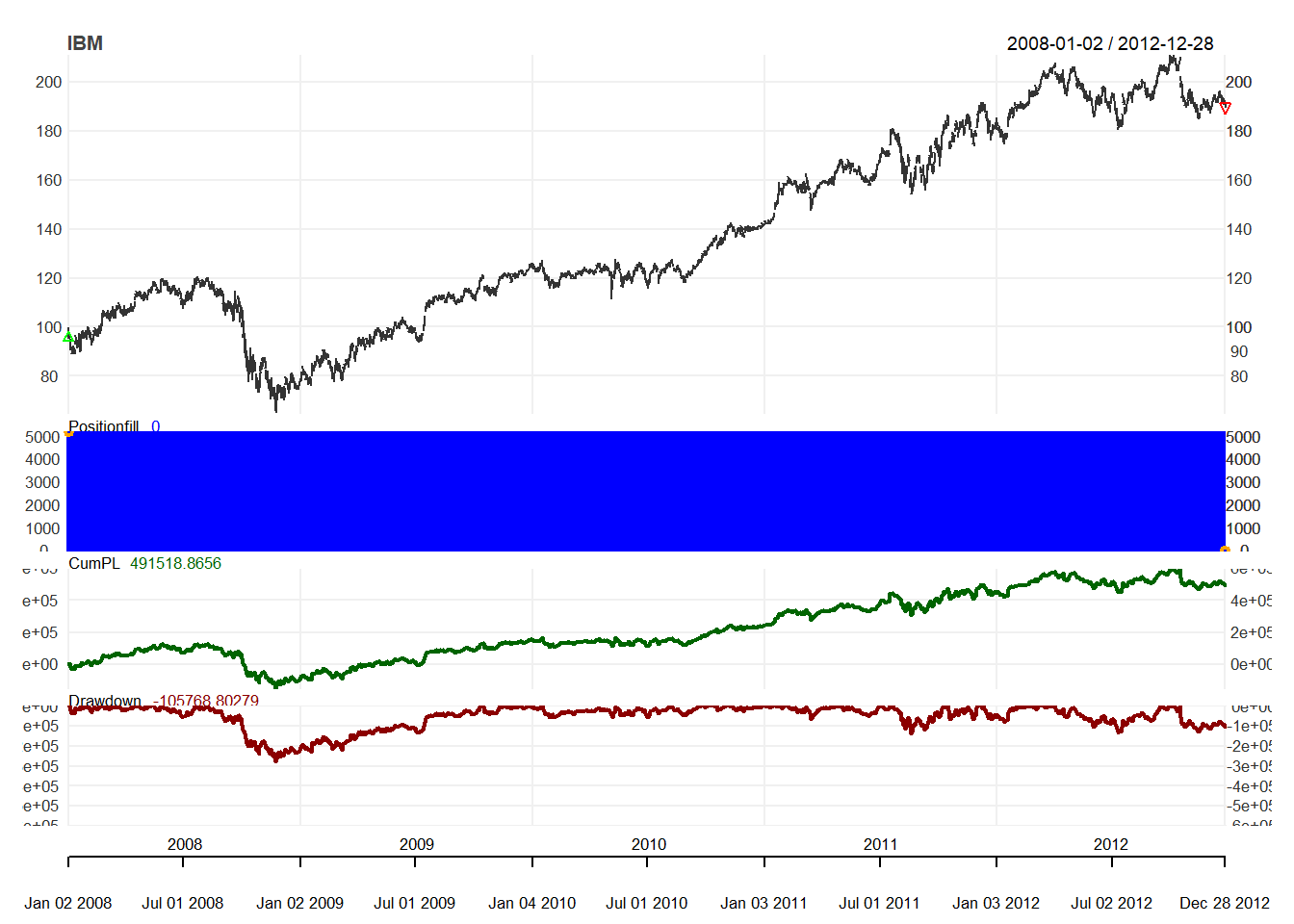
We can see the trading statistics
out <- perTradeStats("buyHold", "IBM")
t(out)
## [,1]
## Start "2008-01-02 08:00:00"
## End "2012-12-28 08:00:00"
## Init.Qty "5223"
## Init.Pos "5223"
## Max.Pos "5223"
## End.Pos "0"
## Closing.Txn.Qty "-5223"
## Num.Txns "2"
## Max.Notional.Cost "499963.2"
## Net.Trading.PL "491518.9"
## MAE "-151359.1"
## MFE "597287.7"
## Pct.Net.Trading.PL "0.98311"
## Pct.MAE "-0.3027405"
## Pct.MFE "1.194663"
## tick.Net.Trading.PL "9410.662"
## tick.MAE "-15135911"
## tick.MFE "59728767"
## duration "157420800 secs"out <- perTradeStats("buyHold", "AAPL")
t(out)## [,1]
## Start "2008-01-02 08:00:00"
## End "2012-12-28 08:00:00"
## Init.Qty "18122"
## Init.Pos "18122"
## Max.Pos "18122"
## End.Pos "0"
## Closing.Txn.Qty "-18122"
## Num.Txns "2"
## Max.Notional.Cost "499972.9"
## Net.Trading.PL "819282.7"
## MAE "-299306.3"
## MFE "1309400"
## Pct.Net.Trading.PL "1.638654"
## Pct.MAE "-0.598645"
## Pct.MFE "2.618941"
## tick.Net.Trading.PL "4520.929"
## tick.MAE "-29930631"
## tick.MFE "130939964"
## duration "157420800 secs"Buy Filter Rule
We use blotter package to apply simple filter rule
buy 1000 units signal if buy signal
hold otherwise
We first Download Data:
from ="2009-01-01"
to ="2012-12-31"
symbols = c("MSFT")
currency("USD")
getSymbols(symbols, from=from, to=to,
           adjust=TRUE)
stock(symbols, currency="USD", multiplier=1)
initEq=10^6
Then setup the account and portfolio:
rm("account.filter",pos=.blotter)
rm("portfolio.filter",pos=.blotter)

initPortf("filter", symbol=symbols)
initAcct("filter", portfolios = "filter",
         initEq = initEq)
Here we generate trading indicator:
price <- Cl(MSFT)
r <- price/Lag(price) - 1
delta<-0.03
signal <-c(NA)
for (i in 2: length(price)){
    if (r[i] > delta){
         signal[i]<- 1
    } else if (r[i]< -delta){
         signal[i]<- -1
    } else
         signal[i]<- 0
}
signal<-reclass(signal,Cl(MSFT))
This convert trading indicator to trading signal:
trade <- Lag(signal)
trade <- na.fill(trade,0)
Now we are ready to apply trading signal into trading action:
for (i in 1:length(price)){
  if (as.numeric(trade[i]) == 1){
    addTxn(Portfolio = "filter",
           Symbol = "MSFT",
           TxnDate = time(price[i]),
           TxnQty = 1000,
           TxnPrice = price[i],
           TxnFees = 0)
  }
    if (as.numeric(trade[i]) == -1){
    addTxn(Portfolio = "filter",
           Symbol = "MSFT",
           TxnDate = time(price[i]),
           TxnQty = -1000,
           TxnPrice = price[i],
           TxnFees = 0)
  }
}
Finally, we update the account and do charting:
updatePortf(Portfolio = "filter")
updateAcct(name = "filter")
updateEndEq(Account = "filter")
chart.Posn("filter", Symbol = "MSFT")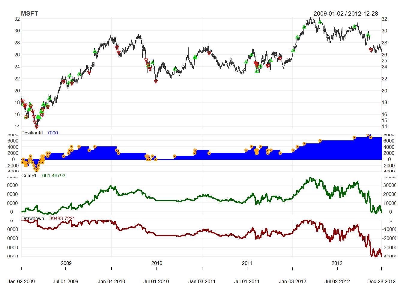
Quanstrat Simple Filter Rule
Step 1: Initialization
We need to install standard packages and custom packages. After loading all the packages, we initialize are variables and then download data.
Then we need to get the data and define initial variables.Download using getSybmols()
options("getSymbols.warning4.0"=FALSE)
from ="2003-01-01"
to ="2012-12-31"
symbols = c("MSFT", "IBM")
getSymbols(symbols, from=from, to=to,
           adjust=TRUE)
Currency is USD for US stocks and the multiplier is always 1 for stocks.
currency("USD")
stock(symbols, currency="USD", multiplier=1)
We first define our strategy, portfolio and account name.
strategy.st <- "filter"
portfolio.st <- "filter"
account.st <- "filter"
Remove any old variables
rm.strat("filter")After naming strategy, portfolio and account, we initialize them:
initEq=100000
initDate="1990-01-01"

initPortf(name=portfolio.st,
          symbols=symbols,
          initDate=initDate,
          currency='USD')
initAcct(name=account.st,
         portfolios=portfolio.st,
         initDate=initDate,
         currency='USD',
         initEq=initEq)
initOrders(portfolio=portfolio.st,
           symbols=symbols,
           initDate=initDate)

strategy(strategy.st, store=TRUE)
Step 2: Define indicator
Indicator is just a function based on price. Since simple filter is not a standard technical indicator, we need to define it first.
filter <- function(price) {
  lagprice <- lag(price,1)
  temp<-price/lagprice - 1
  colnames(temp) <- "filter"
  return(temp)
}
We add the simple filter as an indicator. Here the name is the indicator function we have defined. We need to specify what data to be used by the indicator. Since we have defined that the simple filter rule takes price as input, we need to tell the problem we are using the closing price. Note that the label filter is the variable assigned to this indicator, which implies it must be unique.
add.indicator(
  strategy=strategy.st,
  name = "filter",
  arguments = list(price = quote(Cl(mktdata))),
  label= "filter")
To check if the indicator is defined correctly, use applyindicators to see if it works. The function try() is to allow the program continue to run even if there is an error.
test <-try(applyIndicators(strategy.st,
                           mktdata=OHLC(AAPL)))
head(test, n=4)
Step 3: Trading Signals
Trading signals is generated from the trading indicators. For example, simple trading rule dictates that there is a buy signal when the filter exceeds certain threshold.
In quantstrat, there are three ways one can use a signal. It is refer to as name:
- sigThreshold: more or less than a fixed value
- sigCrossover: when two signals cross over
- sigComparsion: compare two signals
The column refers to the data for calculation of signal. There are five possible relationship:
- gt = greater than
- gte = greater than or equal to
- lt = less than
- lte = less than or equal to
- eq = equal to
Buy Signal under simple trading rule with threshold \(\delta=0.05\)
# enter when filter > 1+\delta
add.signal(strategy.st,
           name="sigThreshold",
           arguments = list(threshold=0.05,
                            column="filter",
                            relationship="gt",
                            cross=TRUE),
           label="filter.buy")
Sell Signal under simple trading rule with threshold \(\delta=-0.05\)
# exit when filter < 1-delta
add.signal(strategy.st,
           name="sigThreshold",
           arguments = list(threshold=-0.05,
                            column="filter",
                            relationship="lt",
                            cross=TRUE),
           label="filter.sell")
Step 4. Trading Rules
While trading signals tell us buy or sell, but it does not specify the execution details.
Trading rules will specify the following seven elements:
- SigCol: Name of Signal
- SigVal: implement when there is signal (or reverse)
- Ordertype: market, stoplimit
- Orderside: long, short
- Pricemethod: market
- Replace: whether to replace other others
- Type: enter or exit the order
Buy rule specifies that when a buy signal appears, place a buy market order with quantity size.
add.rule(strategy.st,
         name='ruleSignal',
         arguments = list(sigcol="filter.buy",
                          sigval=TRUE,
                          orderqty=1000,
                          ordertype='market',
                          orderside='long',
                          pricemethod='market',
                          replace=FALSE),
         type='enter',
         path.dep=TRUE)
Sell rule specifies that when a sell signal appears, place a sell market order with quantity size.
add.rule(strategy.st,
         name='ruleSignal',
         arguments = list(sigcol="filter.sell",
                          sigval=TRUE,
                          orderqty=-1000,
                          ordertype='market',
                          orderside='long',
                          pricemethod='market',
                          replace=FALSE),
         type='enter',
         path.dep=TRUE)
Step 5. Evaluation Results
We will apply the our trading strategy, and the we update the portfolio, account and equity.
out<-try(applyStrategy(strategy=strategy.st,
                       portfolios=portfolio.st))
## [1] "2003-01-21 08:00:00 IBM -1000 @ 69.9146713309017"
## [1] "2005-04-18 08:00:00 IBM -1000 @ 67.691321496698"
## [1] "2007-11-12 08:00:00 IBM -1000 @ 92.7608829720924"
## [1] "2008-01-15 08:00:00 IBM 1000 @ 93.1083408368158"
## [1] "2008-10-02 08:00:00 IBM -1000 @ 96.9042005511082"
## [1] "2008-10-09 08:00:00 IBM -1000 @ 82.3417415861382"
## [1] "2008-10-14 08:00:00 IBM 1000 @ 86.5976050312253"
## [1] "2008-10-16 08:00:00 IBM -1000 @ 84.6732128420016"
## [1] "2008-10-23 08:00:00 IBM -1000 @ 78.0396150349132"
## [1] "2008-10-29 08:00:00 IBM 1000 @ 81.6015883244063"
## [1] "2008-11-14 08:00:00 IBM 1000 @ 74.7358386209428"
## [1] "2008-11-20 08:00:00 IBM -1000 @ 66.7440405789453"
## [1] "2008-11-25 08:00:00 IBM 1000 @ 75.0335538924886"
## [1] "2008-12-02 08:00:00 IBM -1000 @ 74.279956529227"
## [1] "2008-12-09 08:00:00 IBM 1000 @ 76.9314887485928"
## [1] "2009-01-22 08:00:00 IBM 1000 @ 83.7975453378965"
## [1] "2009-03-24 08:00:00 IBM 1000 @ 91.9519343052697"
## [1] "2011-07-20 08:00:00 IBM 1000 @ 179.10642184081"
## [1] "2003-01-21 08:00:00 MSFT -1000 @ 9.73380568942909"
## [1] "2003-02-19 08:00:00 MSFT 1000 @ 18.666511126893"
## [1] "2003-03-14 08:00:00 MSFT 1000 @ 18.9176301004257"
## [1] "2003-04-03 08:00:00 MSFT 1000 @ 19.5796702696815"
## [1] "2003-10-27 08:00:00 MSFT -1000 @ 20.5924922489539"
## [1] "2004-04-26 08:00:00 MSFT 1000 @ 20.8450200245821"
## [1] "2006-05-01 08:00:00 MSFT -1000 @ 21.1026943697531"
## [1] "2007-10-29 08:00:00 MSFT 1000 @ 30.6765128730564"
## [1] "2008-02-04 08:00:00 MSFT -1000 @ 26.8783911230083"
## [1] "2008-04-28 08:00:00 MSFT -1000 @ 25.9103071615352"
## [1] "2008-07-21 08:00:00 MSFT -1000 @ 23.0005500775628"
## [1] "2008-09-18 08:00:00 MSFT -1000 @ 22.7500449360055"
## [1] "2008-09-30 08:00:00 MSFT -1000 @ 24.037954160413"
## [1] "2008-10-01 08:00:00 MSFT 1000 @ 23.8488198695735"
## [1] "2008-10-07 08:00:00 MSFT -1000 @ 20.9217554973638"
## [1] "2008-10-14 08:00:00 MSFT 1000 @ 21.7053081139245"
## [1] "2008-10-15 08:00:00 MSFT -1000 @ 20.4083934382378"
## [1] "2008-10-17 08:00:00 MSFT 1000 @ 21.5522001313782"
## [1] "2008-10-22 08:00:00 MSFT -1000 @ 19.3906765725354"
## [1] "2008-10-29 08:00:00 MSFT 1000 @ 20.7146094033305"
## [1] "2008-11-06 08:00:00 MSFT -1000 @ 18.8052618968231"
## [1] "2008-11-17 08:00:00 MSFT -1000 @ 17.4002718987976"
## [1] "2008-11-20 08:00:00 MSFT -1000 @ 15.8950903484207"
## [1] "2008-11-24 08:00:00 MSFT 1000 @ 18.7603774354557"
## [1] "2008-12-02 08:00:00 MSFT -1000 @ 17.3640024419997"
## [1] "2008-12-09 08:00:00 MSFT 1000 @ 18.6787702509239"
## [1] "2008-12-12 08:00:00 MSFT -1000 @ 17.5544179969251"
## [1] "2008-12-17 08:00:00 MSFT 1000 @ 17.826438016173"
## [1] "2009-01-08 08:00:00 MSFT -1000 @ 18.2435376760854"
## [1] "2009-01-21 08:00:00 MSFT -1000 @ 17.5725509118512"
## [1] "2009-01-23 08:00:00 MSFT -1000 @ 15.595867329838"
## [1] "2009-03-06 08:00:00 MSFT -1000 @ 13.9499293968326"
## [1] "2009-03-11 08:00:00 MSFT 1000 @ 15.6206352048257"
## [1] "2009-03-24 08:00:00 MSFT 1000 @ 16.369256157409"
## [1] "2009-03-27 08:00:00 MSFT 1000 @ 16.5518459433669"
## [1] "2009-04-01 08:00:00 MSFT 1000 @ 17.6291310669443"
## [1] "2009-04-27 08:00:00 MSFT 1000 @ 18.624251288965"
## [1] "2009-07-27 08:00:00 MSFT -1000 @ 21.2323467096564"
## [1] "2009-10-26 08:00:00 MSFT 1000 @ 26.4979519060214"
## [1] "2010-09-14 08:00:00 MSFT 1000 @ 23.5668456416348"
## [1] "2011-08-11 08:00:00 MSFT -1000 @ 24.161608834081"
## [1] "2012-01-23 08:00:00 MSFT 1000 @ 28.912330972876"Now we can update the portfolio, account and equity.
updatePortf(portfolio.st)## [1] "filter"updateAcct(portfolio.st)## [1] "filter"updateEndEq(account.st)## [1] "filter"We can visualize the trading position, profit and loss, and drawdown in graph.
for(symbol in symbols) {
  chart.Posn(Portfolio=portfolio.st,
              Symbol=symbol,
              log=TRUE)
}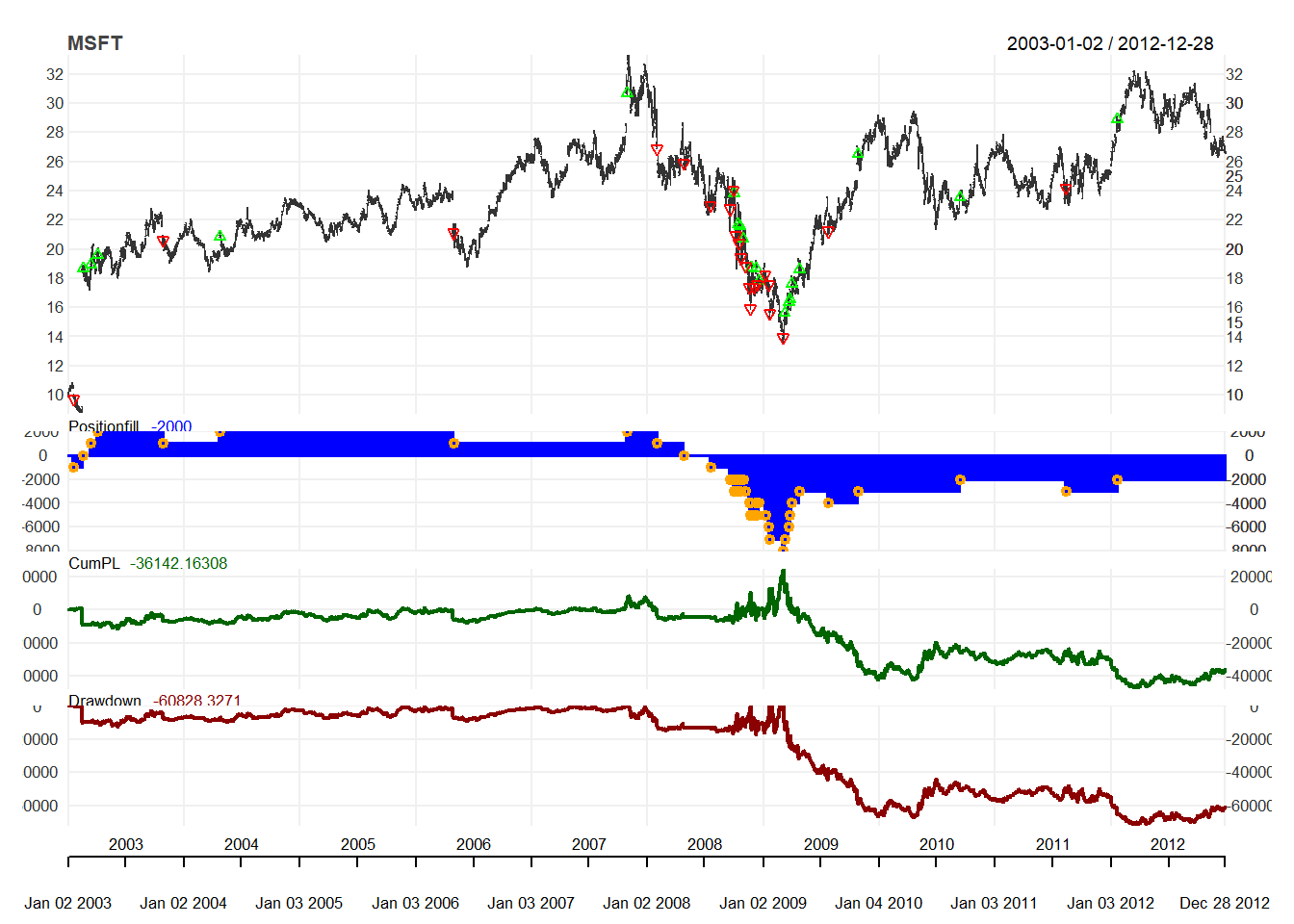
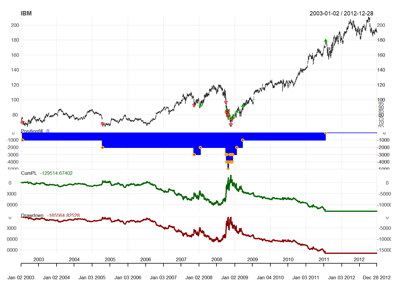
We can also look at the details of the trading statistics of trading strategies such as the number for trades, and profitability of trades.
tstats <- tradeStats(portfolio.st)
t(tstats) #transpose tstats
## IBM MSFT
## Portfolio "filter" "filter"
## Symbol "IBM" "MSFT"
## Num.Txns "18" "42"
## Num.Trades " 9" "20"
## Net.Trading.PL "-129514.67" " -36142.16"
## Avg.Trade.PL "-14390.519" " -1178.172"
## Med.Trade.PL "-3391.6402" " 257.6423"
## Largest.Winner "7730.306" "1715.447"
## Largest.Loser "-101634.719" " -8932.705"
## Gross.Profits "12637.141" " 9785.414"
## Gross.Losses "-142151.81" " -33348.85"
## Std.Dev.Trade.PL "33664.545" " 3514.473"
## Std.Err.Trade.PL "11221.52" " 785.86"
## Percent.Positive "44.44444" "60.00000"
## Percent.Negative "55.55556" "40.00000"
## Profit.Factor "0.08889891" "0.29342583"
## Avg.Win.Trade "3159.2852" " 815.4511"
## Med.Win.Trade "2183.3104" " 780.7065"
## Avg.Losing.Trade "-28430.363" " -4168.606"
## Med.Losing.Trade "-14480.231" " -3272.433"
## Avg.Daily.PL "-14390.519" " -1178.172"
## Med.Daily.PL "-3391.6402" " 257.6423"
## Std.Dev.Daily.PL "33664.545" " 3514.473"
## Std.Err.Daily.PL "11221.52" " 785.86"
## Ann.Sharpe "-6.785846" "-5.321679"
## Max.Drawdown "-167086.24" " -72041.99"
## Profit.To.Max.Draw "-0.7751367" "-0.5016819"
## Avg.WinLoss.Ratio "0.1111236" "0.1956172"
## Med.WinLoss.Ratio "0.1507787" "0.2385707"
## Max.Equity "36050.15" "24686.16"
## Min.Equity "-131036.09" " -47355.83"
## End.Equity "-129514.67" " -36142.16"Then we can evaluate the performance using PerfomanceAnalytics package to see how is the return of the trading strategy.
rets <- PortfReturns(Account = account.st)
rownames(rets) <- NULL
tab <- table.Arbitrary(rets,
                       metrics=c(
                         "Return.cumulative",
                         "Return.annualized",
                         "SharpeRatio.annualized",
                         "CalmarRatio"),
                       metricsNames=c(
                         "Cumulative Return",
                         "Annualized Return",
                         "Annualized Sharpe Ratio",
                         "Calmar Ratio"))
tab
## IBM.DailyEqPL MSFT.DailyEqPL
## Cumulative Return -0.8776990 -0.39612665
## Annualized Return -0.1897894 -0.04926439
## Annualized Sharpe Ratio -0.4801946 -0.29236267
## Calmar Ratio -0.2135370 -0.09109193We can visualize the performance of the trading rule
charts.PerformanceSummary(rets, colorset = bluefocus)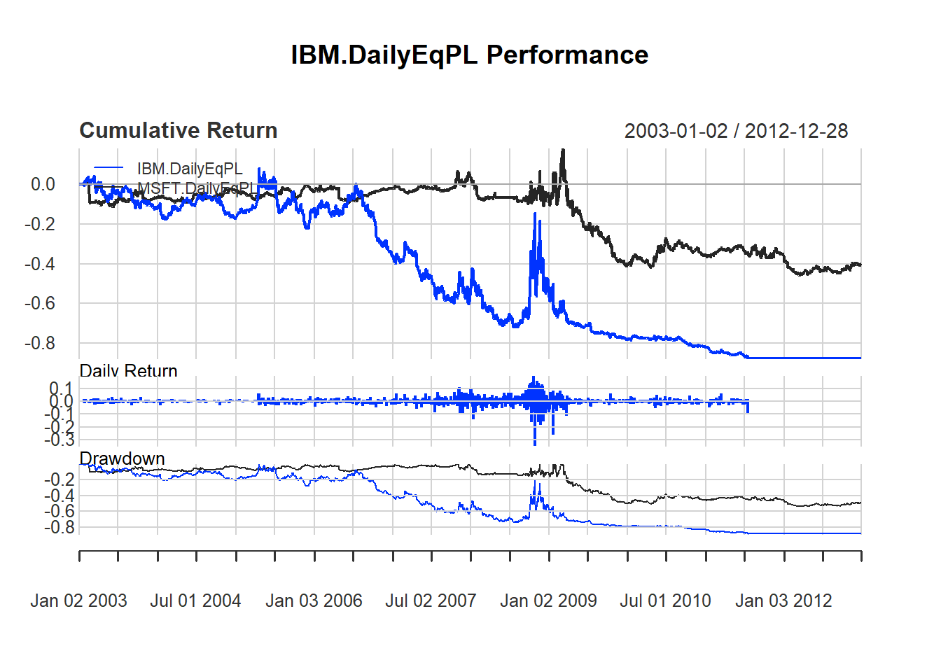
Buy and Hold
We want to compare buy and hold strategy.
We first get the data
getSymbols("SPY", from=from, to=to, adjust=TRUE)Step 1: Initialization
rm.strat("buyHold")

#Initial Setup
initPortf("buyHold", "SPY", initDate = initDate)
initAcct("buyHold", portfolios = "buyHold",
         initDate = initDate, initEq = initEq)
Steps 2-4: Applying trading rule
Since buy and sell are not given by trading rule, we directly add transaction to it.
We first add the transaction to buy at the beginning:
FirstDate <- first(time(SPY))
# Enter order on the first date
BuyDate <- FirstDate
equity = getEndEq("buyHold", FirstDate)
FirstPrice <- as.numeric(Cl(SPY[BuyDate,]))
UnitSize = as.numeric(trunc(equity/FirstPrice))
addTxn("buyHold", Symbol = "SPY",
       TxnDate = BuyDate, TxnPrice = FirstPrice,
       TxnQty = UnitSize, TxnFees = 0)
We first add the transaction to sell at the end:
LastDate <- last(time(SPY))
# Exit order on the Last Date
LastPrice <- as.numeric(Cl(SPY[LastDate,]))
addTxn("buyHold", Symbol = "SPY",
       TxnDate = LastDate, TxnPrice = LastPrice,
       TxnQty = -UnitSize , TxnFees = 0)
Step 5: Evaluation
After updates, we can plot the trading position.
updatePortf(Portfolio = "buyHold")## [1] "buyHold"updateAcct(name = "buyHold")## [1] "buyHold"updateEndEq(Account = "buyHold")## [1] "buyHold"chart.Posn("buyHold", Symbol = "SPY")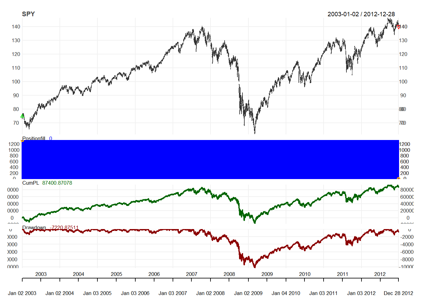
Now we are ready to compare buy-hold and the simple trading rule.
# Compare strategy and market
rets <- PortfReturns(Account = account.st)
rets.bh <- PortfReturns(Account = "buyHold")
returns <- cbind(rets, rets.bh)
charts.PerformanceSummary(
  returns, geometric = FALSE,
  wealth.index = TRUE,
  main = "Strategy vs. Market")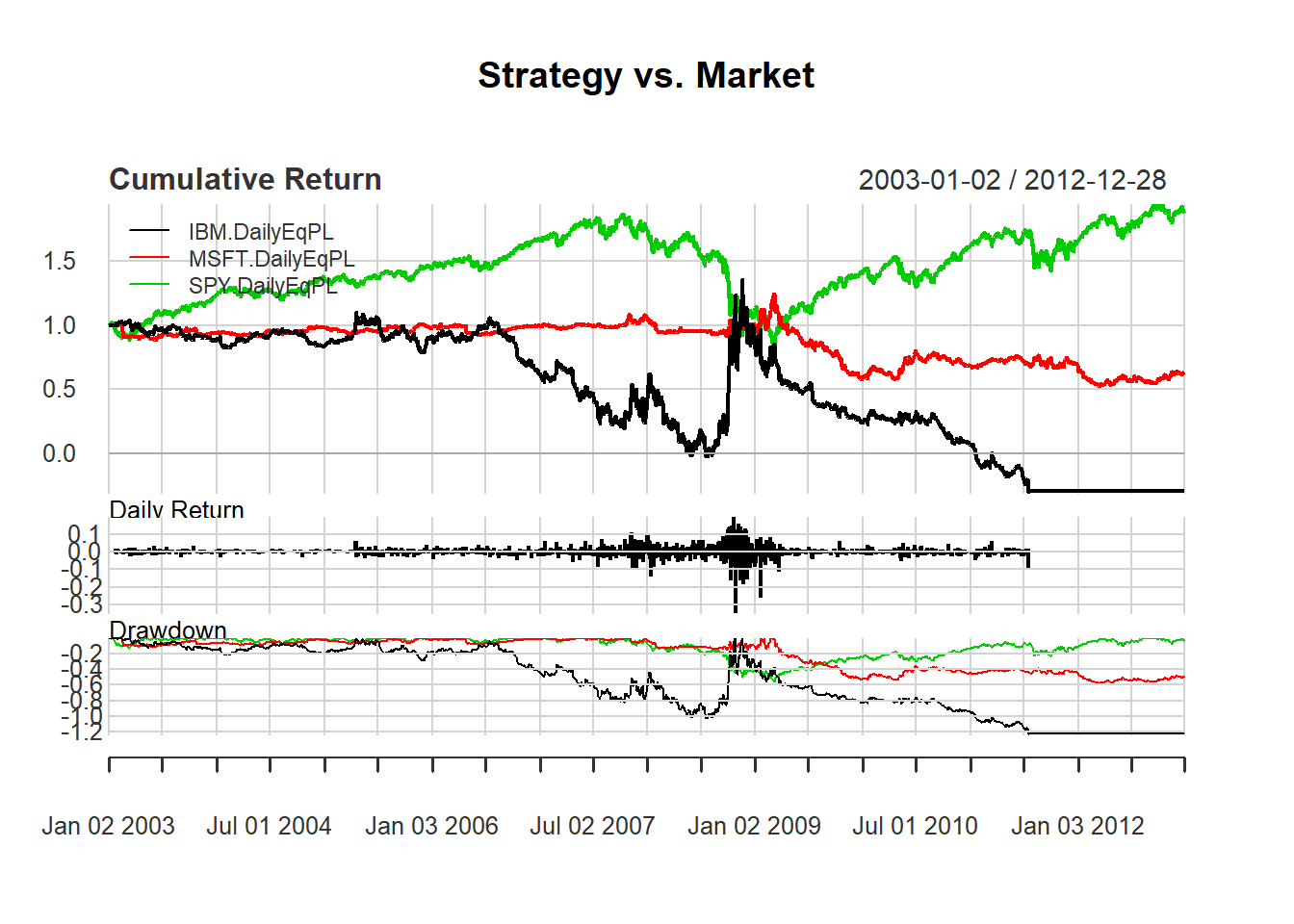
SMA Rule
We will show how to apply the following SMA Rule:
Buy every day when SMA30 SMA200
Sell everything when SMA30 SMA200
Step 1: Initialization
We first initialize the setup.
options("getSymbols.warning4.0"=FALSE)
from ="2012-01-01"
to ="2012-12-31"
symbols = c("IBM","MSFT")
getSymbols(symbols, from=from, to=to,
           adjust=TRUE)
Now we initilized setup:
currency("USD")
strategy.st <- portfolio.st <- account.st <- "SMA"
rm.strat(strategy.st)

initPortf(portfolio.st, symbols)
initAcct(account.st, portfolios=portfolio.st,
         initEq = initEq)
initOrders(portfolio.st)
strategy(strategy.st, store=TRUE)
Step 2: Indicator
Now we add two indicators: SMA30 and SMA200. Here, the argument is different from simple trading rule. For the SMA function, we need to tell the price vector and the number of period.
add.indicator(
  strategy.st, name="SMA",
  arguments=list(x=quote(Cl(mktdata)), n=30),
  label="sma30")

add.indicator(
  strategy.st, name="SMA",
  arguments=list(x=quote(Cl(mktdata)), n=200),
  label="sma200")
Step 3: Signals
Now we add two signals: Buy signal appears when SMA30 is greater than SMA200. Sell signals appears when SMA30 is less than SMA200. Hence, this is different from simple trading rule.
Here, we are going to do signal comparison so that we set name to sigComparison. We will compare two signals: sma30 and sma200. Then the relationship is greater than for buy and less than for less. We name the former to be a buy signal and the latter for a sell signal.
# Bull market if SMA30>SMA200
add.signal(
  strategy.st,
  name="sigComparison",
  arguments=list(columns=c("sma30","sma200"),
                 relationship="gt"),
  label="buy")

# Sell market if SMA30<SMA200
add.signal(
  strategy.st,
  name="sigComparison",
  arguments=list(columns=c("sma30","sma200"),
                 relationship="lt"),
  label="sell")
Note that here we use SigComparsion instead of SigCrossover. It is because SigComparsion will generate signals all the time but SigCrossover will generate signal only at cross.
Step 4: Rules
We will consider buy and sell rules using market order. Note that we sell everything when sell signal arise. Hence, the order quantity is all and the type is exit.
# Buy Rule
add.rule(strategy.st,
         name='ruleSignal',
         arguments = list(sigcol="buy",
                          sigval=TRUE,
                          orderqty=1000,
                          ordertype='market',
                          orderside='long',
                          pricemethod='market',
                          replace=FALSE),
         type='enter',
         path.dep=TRUE)

# Sell Rule
add.rule(strategy.st,
         name='ruleSignal',
         arguments = list(sigcol="sell",
                          sigval=TRUE,
                          orderqty='all',
                          ordertype='market',
                          orderside='long',
                          pricemethod='market',
                          replace=FALSE),
         type='exit',
         path.dep=TRUE)
Step 5: Evaluation
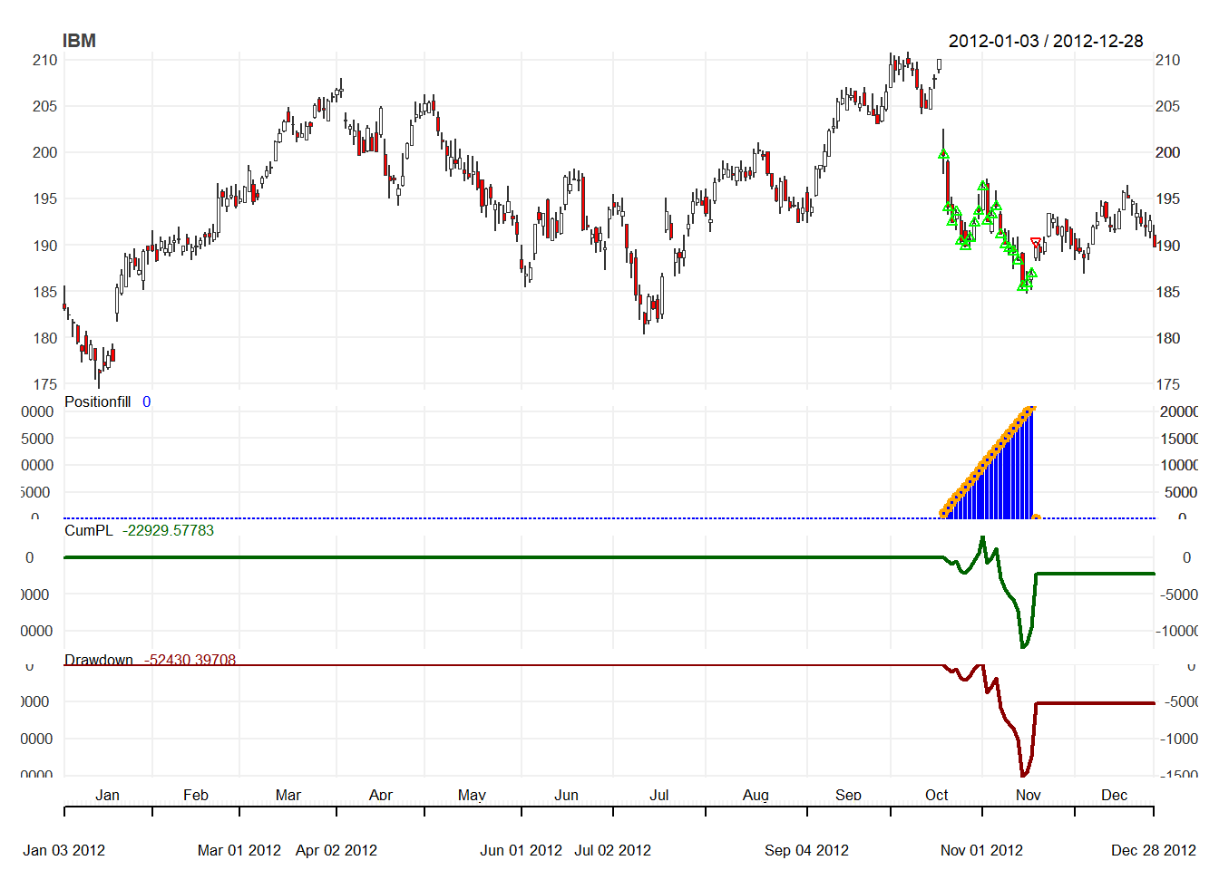
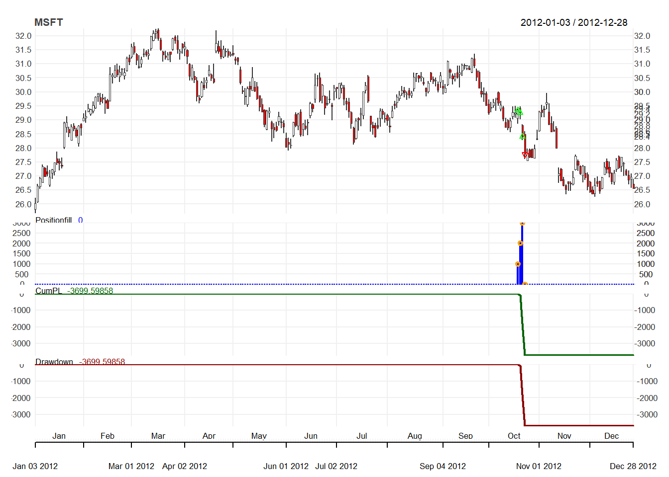
We first try to apply the trading rule.
out<-try(applyStrategy(strategy.st,
                       portfolios=portfolio.st))
## [1] "2012-10-17 08:00:00 IBM 1000 @ 199.755777809092"
## [1] "2012-10-18 08:00:00 IBM 1000 @ 194.1104863151"
## [1] "2012-10-19 08:00:00 IBM 1000 @ 192.517452197251"
## [1] "2012-10-22 08:00:00 IBM 1000 @ 193.552913521349"
## [1] "2012-10-23 08:00:00 IBM 1000 @ 190.416645336717"
## [1] "2012-10-24 08:00:00 IBM 1000 @ 189.888955759662"
## [1] "2012-10-25 08:00:00 IBM 1000 @ 190.765126217072"
## [1] "2012-10-26 08:00:00 IBM 1000 @ 192.42784735108"
## [1] "2012-10-31 08:00:00 IBM 1000 @ 193.682352036262"
## [1] "2012-11-01 08:00:00 IBM 1000 @ 196.290930643838"
## [1] "2012-11-02 08:00:00 IBM 1000 @ 192.58713921341"
## [1] "2012-11-05 08:00:00 IBM 1000 @ 193.294051426163"
## [1] "2012-11-06 08:00:00 IBM 1000 @ 194.220007"
## [1] "2012-11-07 08:00:00 IBM 1000 @ 191.160004"
## [1] "2012-11-08 08:00:00 IBM 1000 @ 190.100006"
## [1] "2012-11-09 08:00:00 IBM 1000 @ 189.639999"
## [1] "2012-11-12 08:00:00 IBM 1000 @ 189.25"
## [1] "2012-11-13 08:00:00 IBM 1000 @ 188.320007"
## [1] "2012-11-14 08:00:00 IBM 1000 @ 185.509995"
## [1] "2012-11-15 08:00:00 IBM 1000 @ 185.850006"
## [1] "2012-11-16 08:00:00 IBM 1000 @ 186.940002"
## [1] "2012-11-19 08:00:00 IBM -21000 @ 190.350006"
## [1] "2012-10-17 08:00:00 MSFT 1000 @ 29.3488341516242"
## [1] "2012-10-18 08:00:00 MSFT 1000 @ 29.2595676739748"
## [1] "2012-10-19 08:00:00 MSFT 1000 @ 28.4065758956973"
## [1] "2012-10-22 08:00:00 MSFT -3000 @ 27.7717930464845"Then we can update the accounts.
updatePortf(portfolio.st)
updateAcct(portfolio.st)
updateEndEq(account.st)
We can also plot the trading positions.
for(symbol in symbols) {
  chart.Posn(Portfolio=portfolio.st,
             Symbol=symbol,log=TRUE)
}
SMA rule with volatility filter
We will consider the following rule:
- Buy every day when
- SMA30 SMA200 and
- 52 period standard deviation of close prices is less than its median over the last N periods.
- Sell everything when
- SMA30 SMA200
Step 1: Initialization
We first download data
from ="2009-01-01"
to ="2012-12-31"
symbols = c("IBM")
currency("USD")
getSymbols(symbols, from=from, to=to, adjust=TRUE)
stock(symbols, currency="USD", multiplier=1)
initEq=10^6
We first initialize the setup.
strategy.st <- portfolio.st <- account.st <- "SMAv"
rm.strat("SMAv")

initPortf(portfolio.st, symbols=symbols,
          initDate=initDate, currency='USD')
initAcct(account.st, portfolios=portfolio.st,
         initDate=initDate, currency='USD',
         initEq=initEq)
initOrders(portfolio.st, initDate=initDate)
strategy(strategy.st, store=TRUE)
Step 2: Indicator
Besides SMA, we will need a new indicator to give buy signal. Since it is combination of SMA and volatility, we need to construct our own indicator, RB:
RB <- function(x,n){
  x <- x
  sd <- runSD(x, n, sample= FALSE)
  med <- runMedian(sd,n)
  mavg <- SMA(x,n)
  signal <- ifelse(sd < med & x > mavg,1,0)
  colnames(signal) <- "RB"
  reclass(signal,x)
  }
Now we are ready to define our indicators:
add.indicator(
  strategy.st, name="SMA",
  arguments=list(x=quote(Cl(mktdata)), n=30),
  label="sma30")

add.indicator(
  strategy.st, name="SMA",
  arguments=list(x=quote(Cl(mktdata)), n=200),
  label="sma200")

add.indicator(
  strategy.st, name="RB",
  arguments=list(x=quote(Cl(mktdata)), n=200),
  label="RB")
Step 3: Signals
Now we add two signals: Buy signal appears when RB is greater than or equal to 1. Sell signals appears when SMA30 is less than SMA200. Hence, this is different from simple trading rule. Here, we are going to do signal comparison. There are two price lists: sma200 and sma30. Then the relationship is greater than for buy and less than for less.
# Bull market if RB>=1
add.signal(strategy.st,
           name="sigThreshold",
           arguments = list(threshold=1, column="RB",
                            relationship="gte",
                            cross=TRUE),
           label="buy")

# Sell market if SMA30<SMA200
add.signal(strategy.st,
           name="sigComparison",
           arguments=list(columns=c("sma30","sma200"),
                          relationship="lt"),
           label="sell")
Step 4: Rules
We now consider buy and sell rules using market order. Note that this is the same as the case for simple SMA rule.
# Buy Rule
add.rule(strategy.st,
name='ruleSignal',
arguments = list(sigcol="buy",
sigval=TRUE,
orderqty=1000,
ordertype='market',
orderside='long',
pricemethod='market',
replace=FALSE),
type='enter',
path.dep=TRUE)
# Sell Rule
add.rule(strategy.st,
name='ruleSignal',
arguments = list(sigcol="sell",
sigval=TRUE,
orderqty='all',
ordertype='market',
orderside='long',
pricemethod='market',
replace=FALSE),
type='exit',
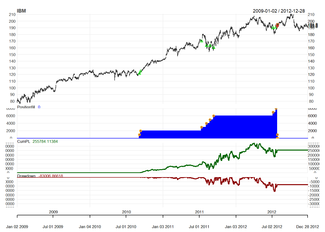
path.dep=TRUE) Step 5: Evaluation
We first try to apply the trading rule.
out<-try(applyStrategy(strategy.st,
                       portfolios=portfolio.st))
## [1] "2010-09-07 08:00:00 IBM 1000 @ 121.265927698413"
## [1] "2010-09-13 08:00:00 IBM 1000 @ 124.789816471828"
## [1] "2011-07-14 08:00:00 IBM 1000 @ 169.919478248927"
## [1] "2011-08-08 08:00:00 IBM 1000 @ 162.813574456635"
## [1] "2011-08-24 08:00:00 IBM 1000 @ 163.342502099495"
## [1] "2011-09-13 08:00:00 IBM 1000 @ 160.080743434437"
## [1] "2012-07-06 08:00:00 IBM 1000 @ 189.765720727769"
## [1] "2012-07-20 08:00:00 IBM 1000 @ 190.796779800297"
## [1] "2012-07-26 08:00:00 IBM -8000 @ 192.283894241252"
## [1] "2012-07-27 08:00:00 IBM 1000 @ 194.702935714691"
## [1] "2012-07-30 08:00:00 IBM -1000 @ 194.990438558152"Then we can update the accounts.
updatePortf(portfolio.st)
updateAcct(portfolio.st)
updateEndEq(account.st)
We can also plot the trading positions.
chart.Posn(Portfolio=portfolio.st,
           Symbol="IBM",
           log=TRUE)