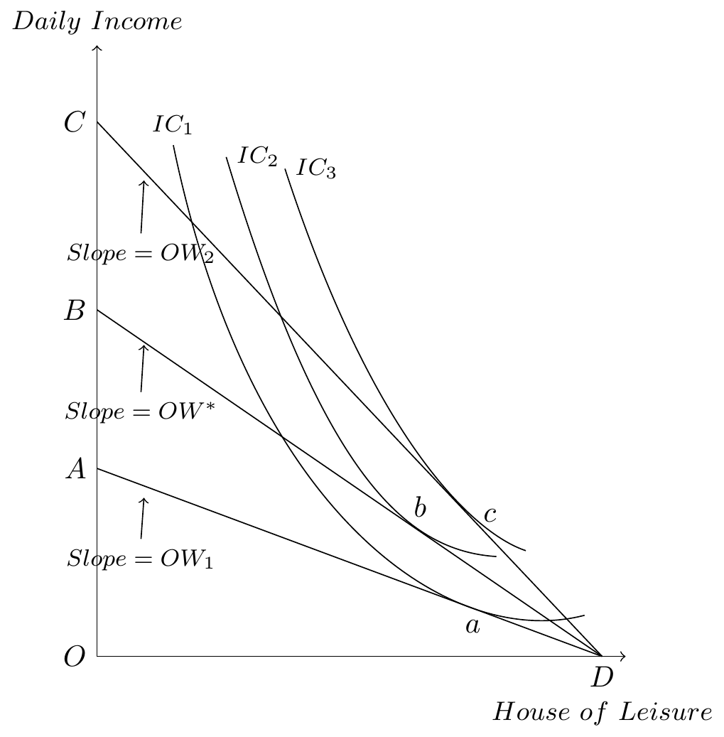
Labor Supply Decision
\begin{tikzpicture}[scale=0.7]
\draw [<->] (0,10.4) node [above] {\small $Daily\ Income$} --(0,0) node [left] {$O$} --(9,0);
\node [below] at (8.6, -0.6) {\small $House\ of\ Leisure$};
\node [left] at (0,3.2) {$A$};
\node [left] at (0,5.9) {$B$};
\node [left] at (0,9.1) {$C$};
\node [below] at (8.6,0) {$D$};
\node [below] at (6.4,0.8) {$a$};
\node [above] at (5.5,2.2) {$b$};
\node [right] at (6.4,2.4) {$c$};
% Slope OW
\draw (0,3.2)--(8.6,0);
\draw (0,5.9)--(8.6,0);
\draw (0,9.1)--(8.6,0);
\draw [->] (0.75,2) node [below] {\footnotesize$Slope = OW_1$}--(0.8,2.7);
\draw [->] (0.75,4.5) node [below] {\footnotesize$Slope = OW^*$} --(0.8,5.3);
\draw [->] (0.75,7.2) node [below] {\footnotesize$Slope = OW_2$} --(0.8,8.1);
% ICs
\draw (1.3,8.7) node [above] {\footnotesize$IC_1$} ..controls (2.6,2.4) and (6,0.1) ..(8.3,0.7);
\draw (2.2,8.5) node [right] {\footnotesize$IC_2$} ..controls (3.8,3.2) and (5.2,1.8) ..(6.8,1.7);
\draw (3.2,8.3) node [right] {\footnotesize$IC_3$} ..controls (4.7,3.7) and (6.4,2.1) ..(7.3,1.8);
\end{tikzpicture}
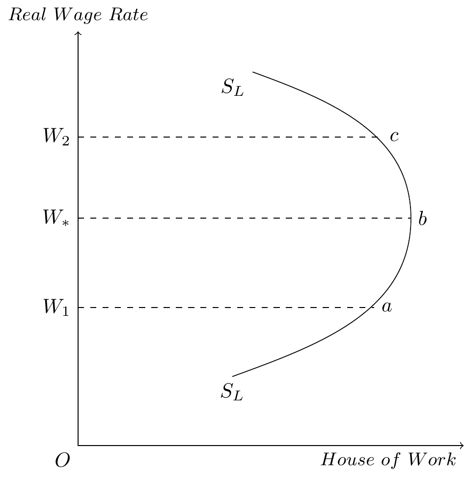
Labor Supply Curve
\begin{tikzpicture}[scale=0.7]
\draw [<->] (0,10.2) node [above] {\small $Real\ Wage\ Rate$} --(0,0) node [below left] {$O$}--(9.5,0) node [below left] {\small $House\ of\ Work$};
\node [left] at (0,3.4) {$W_1$};
\node [left] at (0,5.6) {$W_*$};
\node [left] at (0,7.6) {$W_2$};
\node [right] at (7.3,3.4) {$a$};
\node [right] at (8.2,5.6) {$b$};
\node [right] at (7.5,7.6) {$c$};
\draw [dashed] (0,3.4)--(7.3,3.4);
\draw [dashed] (0,5.6)--(8.2,5.6);
\draw [dashed] (0,7.6)--(7.4,7.6);
\draw (3.8,1.7) node [below] {$S_L$} to [out=20, in=-90] (8.2,5.6) to [out=90, in=-20] (4.3,9.2) node [below left] {$S_L$};
\end{tikzpicture}
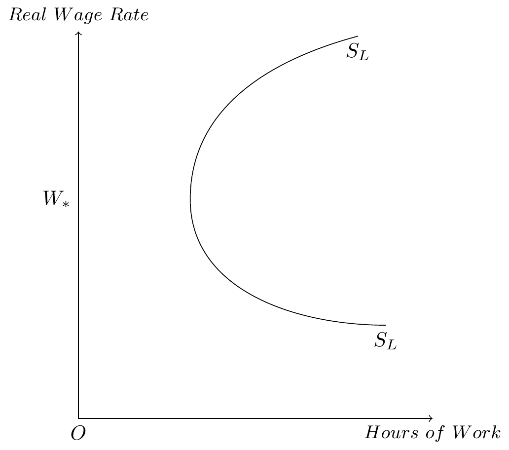
Backward Bending Labor Supply Curve
\begin{tikzpicture}[scale=0.8]
\draw [<->] (0,8.3) node [above] {\small $Real \ Wage \ Rate$} --(0,0) node [below] {$O$}--(7.6,0) node [below] {\small $Hours \ of \ Work$};
\node [left] at (0,4.7){$W_*$};
\draw (6,8.2)node [below] {$S_L$} to [out=-165, in=90] (2.4, 4.7) to [out=-90, in=180] (6.6,2) node [below] {$S_L$};
\end{tikzpicture}
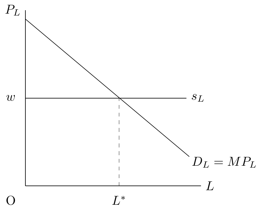
Labor Demand and Supply
\begin{tikzpicture}[scale=0.8]
\draw (0,0) -- (6,0) node [right] {$L$};
\draw (0,0) -- (0,6) node [left] {$P_L$};
\node at (-0.5,-0.5) {O};
\draw (0,3)--(5.5,3);
\node at (5.9,3) {$s_L$};
\node at (-0.5,3) {$w$};
\draw (0,5.7)--(5.6,1);
\node at (6.8,0.8) {$D_L=MP_L$};
\draw[dashed](3.2,0)--(3.2,3.1);
\node at (3.2,-0.5) {$L^{*}$};
\end{tikzpicture}
Income distribution
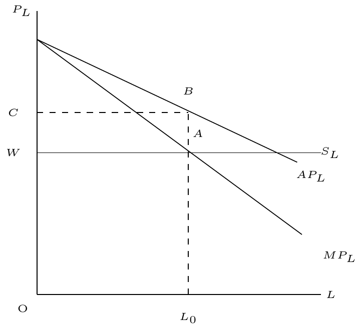
\begin{tikzpicture}[scale=0.8]
\tiny
\draw (0,0) -- (6,0) node [right] {$L$};
\draw (0,0) -- (0,6) node [left] {$P_L$};
\node at (-0.3,-0.3) {O};
\draw (0,3)--(6,3);
\node at (6.2,3) {$S_L$};
\node at (-0.5,3) {$W$};
\draw (0,5.4)--(5.6,1.27);
\node at (3.4,3.4) {$A$};
\node at (6.4,0.8) {$MP_L$};
\draw[dashed](3.2,0)--(3.2,3.85);
\node at (-0.5,3.85) {$C$};
\node at (3.2,4.3) {$B$};
\draw[dashed](0,3.85)--(3.2,3.85);
\node at (3.2,-0.5) {$L_0$};
\draw (0,5.4)--(5.5,2.8);
\node at (5.8,2.5) {$AP_L$};
\end{tikzpicture}