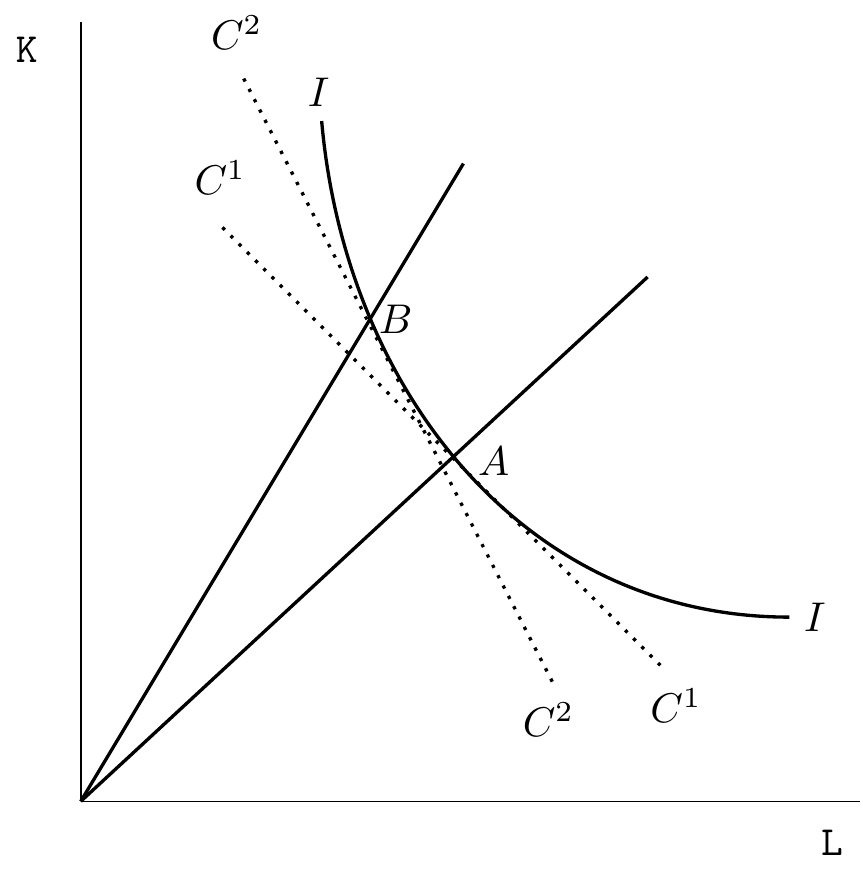
Isoquant
\begin{tikzpicture}[scale=1.2]
\draw (0,0) -- (5.5,0);
\draw (0,0) -- (0,5.5);
\node [left] at (-0.2,5.3) {$\texttt{K}$};
\node [below] at (5.3,-0.1) {$\texttt{L}$};
\draw [thick] (1.7,4.8) to [out=275,in=180] (5,1.3);
\node [right] at (1.5,5) {$I$};
\node [right] at (5,1.3) {$I$};
\draw [thick] (0,0) -- (2.7,4.5);
\draw [thick] (0,0) -- (4,3.7);
\draw[dotted, thick](1,4.05)--(4.1,0.95);
\draw[dotted, thick](1.15,5.1)--(3.35,0.8);
\node [right] at (0.7,4.4) {$C^1$};
\node [below] at (4.2,0.9) {$C^1$};
\node [above] at (1.1,5.2) {$C^2$};
\node [below] at (3.3,0.8) {$C^2$};
\node [right] at (2,3.4) {$B$};
\node [right] at (2.7,2.4) {$A$};
\end{tikzpicture}
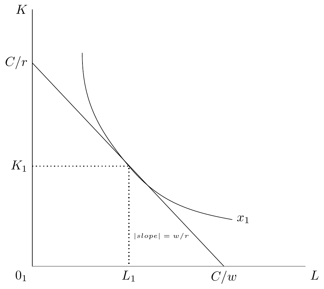
Cost Minimization
\begin{tikzpicture}[scale=.9]
\draw (0,7.7) node [left] {$K$} -- (0,0) node [below left] {$0_1$} -- (8.2,0) node [below right] {$L$};
\node [left] at (0,6.1) {$C/r$};
\node [below] at (5.75,0) {$C/w$};
\node [below] at (2.9,0) {$L_1$};
\node [left] at (0,3) {$K_1$};
\node [right] at (6,1.4) {$x_1$};
\node [right] at (2.9,.9) {\tiny $|slope|=w/r$};
\draw [dotted, thick] (0,3) -- (2.9,3) -- (2.9,0);
\draw (1.5,6.4) to [out=-90, in=130] (2.9,3) to [out=-50, in=170] (6,1.4);
\draw (0,6.1) -- (5.75,0);
\end{tikzpicture}
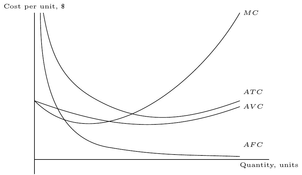
Short-run Cost Curves
\begin{tikzpicture}[scale=0.8]
\tiny
\draw (0,0) -- (8,0) node [below] {Quantity, units};
\draw (0,-0.5) -- (0,5) node [above] {Cost per unit, \$};
\draw (0.2,5) to [out=270,in=172] (2.6,0.4);
\draw (2.6,0.4) to [out=350.5,in=178] (7,0.1);
\node [right] at (7,0.5) {$AFC$};
\draw (0.3,5) to [out=280,in=150] (2,2.1);
\draw (2,2.1) to [out=330,in=200] (7,2);
\node [right] at (7,2.3) {$ATC$};
\draw (0,2) to [out=340,in=200] (7,1.8);
\node [right] at (7,1.8) {$AVC$};
\draw (0,2) to [out=315,in=240] (7,5);
\node [right] at (7,5) {$MC$};
\end{tikzpicture}
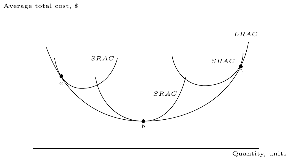
Long-run Cost Curves
\begin{tikzpicture}[scale=0.8]
\tiny
\draw (-0.3,0)-- (0,0) -- (8,0) node [below] {Quantity, units};
\draw (0,-0.5)-- (0,0) -- (0,5) node [above] {Average total cost, \$};
\draw (0.2,3.7) to [out=290,in=180] (3.75,1);
\draw (3.75,1) to [out=360,in=260] (7.6,3.9);
\node [above] at (7.5,4) {$LRAC$};
\draw (0.5,3.3) to [out=280,in=180] (1.5,2.2);
\draw (1.5,2.2) to [out=360,in=255] (2.8,3.3);
\draw [fill] (0.75,2.65) circle [radius =0.06];
\node [below] at (0.75,2.55){$a$};
\node [left] at (2.8,3.3){$SRAC$};
\draw (2,2.6) to [out=280,in=180] (3.75,1);
\draw (3.75,1) to [out=360,in=255] (5.3,2.6);
\draw [fill] (3.75,1) circle [radius =0.06];
\node [below] at (3.75,1) {$b$};
\node [left] at (5.1,2) {$SRAC$};
\draw (4.8,3.4) to [out=280,in=180] (6,2.3);
\draw (6,2.3) to [out=360,in=270] (7.4,3.5);
\draw [fill] (7.32,3) circle [radius =0.06];
\node [below] at (7.32,3) {$c$};
\node [left] at (7.22,3.2) {$SRAC$};
\end{tikzpicture}
Production Possibility Frontier
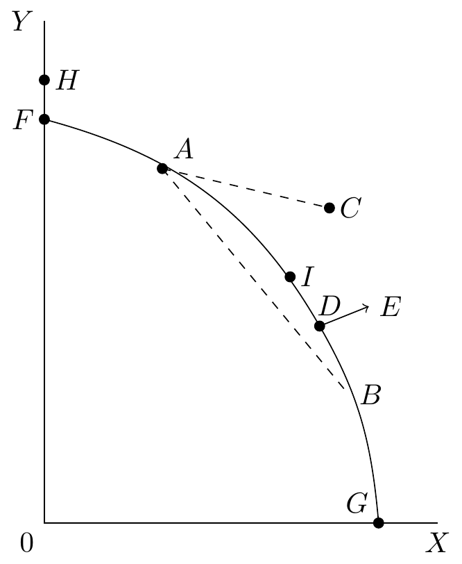
\begin{tikzpicture}[scale=1.2]
\draw (0,5.1) node [left] {$Y$} -- (0,0) node [below left] {$0$} -- (4,0) node [below] {$X$};
\draw (0,4.1) to [out=-15, in=120] (2.8,2) to [out=-60, in=95] (3.4,0);
\draw [->] (2.8,2) -- (3.3,2.2);
\draw [dashed] (1.2,3.6) -- (3.1,1.3);
\draw [dashed] (1.2,3.6) -- (2.9,3.2);
\node [right] at (3.3,2.2) {$E$};
\node [right] at (3.1,1.3) {$B$};
\node [left] at (0,4.1) {$F$};
\draw [fill] (0,4.1) circle [radius=.05];
\node [right] at (0,4.5) {$H$};
\draw [fill] (0,4.5) circle [radius=.05];
\node [above left] at (3.4,0) {$G$};
\draw [fill] (3.4,0) circle [radius=.05];
\node [right] at (2.5,2.5) {$I$};
\draw [fill] (2.5,2.5) circle [radius=.05];
\node [above] at (2.9,2) {$D$};
\draw [fill] (2.8,2) circle [radius=.05];
\node [right] at (2.9,3.2) {$C$};
\draw [fill] (2.9,3.2) circle [radius=.05];
\node [above right] at (1.2,3.6) {$A$};
\draw [fill] (1.2,3.6) circle [radius=.05];
\end{tikzpicture}